Chapter 11 — Neural Radiance Fields (NeRF)¶
Exam weight: ~10 / 110 points in the trial exam (Q10: five True/False statements about what a NeRF is, what it needs for training, and how it renders). These are among the cheapest points in the whole exam — if you can recite the scene function, the volume-rendering equation, and the training requirements without hesitation. Beginner-friendly, math-deep notes for the SS 2025 CVML exam at TU Braunschweig.
§1 Chapter Roadmap¶
A Neural Radiance Field (NeRF) is a small fully-connected neural network that memorizes an entire 3-D scene as a single continuous function: feed in a 3-D position and a viewing direction, \(F_\Theta (x, y, z, \theta , \phi )\), and it returns a color and a density, \((r, g, b, \sigma )\). There is no mesh, no voxel grid, no texture — the whole scene lives implicitly in a few megabytes of network weights. To render a new view, you shoot a ray from the camera through each pixel, sample points along the ray, query the network at every sample, and blend the answers front-to-back with the classic volume-rendering equation \(C(r) = \int T(t)\cdot \sigma (t)\cdot c(t, d) dt\) — exactly the alpha compositing used for decades to visualize CT and MRI scans. Training is brutally simple: render rays, compare against the real photo pixels with a squared error, and backpropagate. The magic that makes it work comes from three intricacies stressed in the lecture: (1) positional encoding \(\gamma (p)\) lifts the 5-D input into sin/cos frequency bands, defeating the MLP's spectral bias toward low-frequency (cartoony) functions; (2) the view direction enters only at the penultimate layer, forcing most of the network to learn view-independent geometry and avoiding the shape-radiance ambiguity; (3) hierarchical sampling spends a coarse pass finding where the scene actually is, then importance-samples fine points there. This chapter connects backward to Chapter 10 (NeRF needs camera poses from SfM/COLMAP and the ray math from calibration) and forward to the post-NeRF world (instant-NGP, 3D Gaussian Splatting).
বাংলা: Neural Radiance Field (NeRF) হলো একটা ছোট fully-connected neural network, যেটা পুরো একটা 3-D scene-কে একটাই continuous function হিসেবে মুখস্থ করে রাখে: input দিন একটা 3-D position আর একটা viewing direction — \(F_\Theta (x, y, z, \theta , \phi )\) — আর output পাবেন একটা color ও একটা density — \((r, g, b, \sigma )\)। এখানে কোনো mesh নেই, voxel grid নেই, texture নেই — পুরো scene-টা থাকে network-এর weight-গুলোর ভেতরে, implicit ভাবে। নতুন view render করতে হলে camera থেকে প্রতিটা pixel-এর ভেতর দিয়ে একটা ray পাঠান, ray-এর উপর কিছু sample point নিন, প্রতিটা point-এ network-কে জিজ্ঞেস করুন "এখানে রঙ কী, density কত?", তারপর উত্তরগুলোকে সামনে-থেকে-পেছনে volume rendering দিয়ে মিশিয়ে একটা pixel color বানান — ঠিক যেভাবে CT/MRI scan visualize করা হয়। Training আরও সহজ: render করা রঙ আর আসল ছবির রঙের পার্থক্যের squared error কমান। কিন্তু কাজ করানোর আসল জাদু তিনটা: (১) positional encoding — sin/cos frequency band দিয়ে input-কে উঁচু dimension-এ তোলা, যাতে MLP-র low-frequency (cartoon-এর মতো) শেখার প্রবণতা (spectral bias) কাটে; (২) viewing direction ঢোকে একদম শেষের আগের (penultimate) layer-এ — তাই network-এর বেশিরভাগ অংশ শুধু geometry শেখে; (৩) hierarchical sampling — আগে মোটা দাগে খুঁজে নাও scene কোথায়, তারপর সেখানেই বেশি sample দাও। Chapter 10-এর সাথে সরাসরি যোগ: NeRF-এর camera pose আসে SfM/COLMAP থেকে।
§2 Concepts from Zero¶
2.1 The problem: novel view synthesis¶
Given a set of photos of a scene taken from known camera positions, produce a photo-realistic image of the same scene from a camera position nobody ever photographed. That is novel view synthesis. Chapter 9's view morphing interpolates between two images; Chapter 10's reconstruction builds explicit 3-D geometry. NeRF takes a third path: it learns a function that can answer "what does this point look like from this direction?" for every point in space — so any new camera view can be rendered by just asking the function many times.
বাংলা: Novel view synthesis মানে: একটা scene-এর কিছু ছবি (যাদের camera position জানা) থেকে এমন একটা নতুন ছবি বানানো, যে জায়গা থেকে কেউ কখনো ছবি তোলেইনি — অথচ ছবিটা দেখতে হবে আসল ফটোর মতো। Chapter 9-এর view morphing দুটো ছবির মাঝে interpolate করে, Chapter 10 explicit 3-D geometry বানায়। NeRF তৃতীয় পথ নেয়: সে এমন একটা function শেখে যেটা space-এর যেকোনো point সম্পর্কে বলতে পারে "এই দিক থেকে দেখলে এটা কেমন দেখায়" — তাই নতুন যেকোনো camera-র জন্য শুধু function-টাকে অনেকবার জিজ্ঞেস করলেই ছবি তৈরি।
2.2 Two roads to rendering: physics-based vs image-based¶
- Physics-based rendering (classic computer graphics): model the geometry, assign materials, place lights, then solve the rendering equation (usually with Monte Carlo path tracing). Photo-realistic — the movie industry's approach — but it needs hand-made 3-D assets and costs enormous compute.
- Image-based rendering: skip the 3-D model; capture images of the real scene and interpolate between them. The lecture's history: the Wing Commander game (pre-rendered spaceship sprites from many angles, shown by nearest view) even before QuickTime VR; later light fields, Photo Tourism (1,275 community photos of St. Peter's Basilica — navigable but full of artifacts, not photo-realistic), and now NeRF. The two worlds converge in modern games: hand-made geometry (flexible for animation/physics) plus image-based materials captured with rigs like the Stanford light gantry (camera + lamp orbiting a material sample).
NeRF is image-based rendering's current crown: it produces photo-realistic novel views from photos alone.
বাংলা: Rendering-এর দুটো রাস্তা। Physics-based: geometry বানাও, material লাগাও, আলো বসাও, তারপর rendering equation solve করো (Monte Carlo path tracing) — সিনেমার পদ্ধতি, ফল photo-realistic কিন্তু সবকিছু হাতে বানাতে হয় আর খরচ বিশাল। Image-based: 3-D model বাদ; আসল scene-এর ছবি তুলে ছবিগুলোর মাঝে interpolate করো — Wing Commander game, QuickTime VR, light field, Photo Tourism (১,২৭৫টা ছবি দিয়ে St. Peter's Basilica — চলাফেরা করা যায় কিন্তু artifact-ভরা), আর এখন NeRF। আধুনিক game-এ দুটো জগৎ মিশে গেছে: geometry হাতে বানানো (animation-এর সুবিধার জন্য), কিন্তু material/texture আসল জগৎ থেকে ক্যাপচার করা। NeRF হলো image-based পথের বর্তমান মুকুট — শুধু ছবি থেকেই photo-realistic নতুন view।
2.3 The rendering equation in one breath¶
Physics-based rendering answers: what radiance leaves point x in direction \(\omega _{o}\)?
- \(L_{e}\) — self-emission (nonzero only for light sources).
- The integral — over the whole hemisphere \(\Omega\) around
x: all incoming light \(L_{i}\) from every direction \(\omega _{i}\), scaled by the material's reflectance function \(f_{r}\) (the BRDF: what fraction of light from \(\omega _{i}\) bounces toward \(\omega _{o}\)) and by the surface-alignment factor \(\cos \theta _{i}\).
NeRF bypasses this equation entirely: instead of simulating light transport, it directly fits a function to the observed outgoing radiance. Lighting, materials, and shadows are all baked into the learned colors.
বাংলা: Rendering equation প্রশ্নটার উত্তর দেয়: point x থেকে direction \(\omega _{o}\)-তে কতটুকু আলো (radiance) বের হয়? উত্তর = নিজের emission (\(L_{e}\), শুধু আলোর উৎসে nonzero) + hemisphere-এর সব দিক থেকে আসা আলোর integral, যেখানে material-এর BRDF \(f_{r}\) বলে দেয় কোন দিকের আলোর কত ভাগ আমার দিকে প্রতিফলিত হবে, আর \(\cos \theta _{i}\) বলে surface কতটা আলোর দিকে ঘোরানো। NeRF এই পুরো হিসাবটাই এড়িয়ে যায়: আলো simulate না করে সে সরাসরি observed radiance-এ একটা function fit করে — আলো, ছায়া, material সব শেখা রঙের ভেতরে "বেক" হয়ে থাকে।
2.4 Volume rendering — NeRF's real ancestor¶
NeRF's idea comes not from classic surface rendering but from volume rendering of medical data. An MRI/CT scanner records slices; stacked, they form a 3-D grid of voxels (volume elements), each storing attributes — density at minimum, optionally color. To view the volume:
- Ray casting — shoot a ray from the camera through each pixel into the volume.
- Sampling — pick sample positions along the ray inside the volume.
- Shading — evaluate the attributes (via a transfer function mapping attributes to color/opacity) at each sample.
- Compositing — blend the samples front-to-back with alpha blending.
The lecture's sampling caveat: step too coarsely and you skip voxels → information loss → aliasing artifacts. By the Nyquist theorem the sampling rate should be at least twice the highest frequency in the volume — worst case, a step size of about one voxel.
NeRF keeps steps 1–4 unchanged and replaces only the voxel grid: instead of looking attributes up in a stored 3-D array, it asks a neural network.
বাংলা: NeRF-এর আসল পূর্বপুরুষ হলো medical data-র volume rendering। MRI/CT scanner স্তরে স্তরে slice তোলে; slice-গুলো জমালে পাওয়া যায় voxel-এর (volume element) একটা 3-D grid — প্রতিটা voxel-এ থাকে density (চাইলে রঙও)। দেখার নিয়ম চার ধাপে: (১) ray casting — camera থেকে প্রতিটা pixel দিয়ে ray ছোড়া; (২) sampling — ray-এর উপর sample position বাছা; (৩) shading — transfer function দিয়ে attribute থেকে রঙ/opacity বের করা; (৪) compositing — সামনে-থেকে-পেছনে alpha blending। সাবধানতা: sample-এর ফাঁক বেশি হলে voxel বাদ পড়ে → তথ্য হারায় → aliasing; Nyquist theorem অনুযায়ী sampling-এর হার সর্বোচ্চ frequency-র অন্তত দ্বিগুণ হওয়া চাই (worst case: ধাপ ≈ এক voxel)। NeRF এই চার ধাপ হুবহু রেখে শুধু voxel grid-টা বদলে দেয় — table lookup-এর জায়গায় neural network-কে প্রশ্ন।
2.5 What a NeRF is: a scene as a 5-D function¶
A NeRF is a multi-layer perceptron (MLP) — a plain fully-connected network, in the original paper 9 layers with 256 channels each — that implements
Five numbers in: the 3-D position of a query point and the direction you are looking from (two angles in polar coordinates — a unit 3-D vector works too, but two angles avoid redundancy). Four numbers out: the emitted color at that point as seen from that direction, and the volume density \(\sigma\) — how opaque the point is, independent of direction. The network "memorizes the scene as a function." Mental model from the lecture: a 3-D colored fog stored in network weights. Ask anywhere, it answers; ask along a ray and composite, and you get a photograph.
বাংলা: NeRF হলো একটা সাধারণ multi-layer perceptron (MLP) — fully-connected network, মূল paper-এ ৯টা layer, প্রতিটায় ২৫৬টা channel — যেটা function-টা বাস্তবায়ন করে: \(F_\Theta : (x, y, z, \theta , \phi ) \to (r, g, b, \sigma )\)। Input পাঁচটা সংখ্যা: point-এর 3-D position আর কোন দিক থেকে দেখছি (polar coordinate-এ দুটো কোণ; 3-D unit vector-ও চলে, কিন্তু দুটো কোণে redundancy কম)। Output চারটা সংখ্যা: ওই দিক থেকে দেখা রঙ (r, g, b) আর volume density \(\sigma\) — point-টা কতটা অস্বচ্ছ (এটা দিক-নিরপেক্ষ)। মনে রাখার ছবি: network-এর weight-এর ভেতরে রাখা একটা রঙিন 3-D কুয়াশা — যেখানে খুশি প্রশ্ন করো, উত্তর পাবে; একটা ray বরাবর প্রশ্ন করে উত্তরগুলো মেশালে একটা ফটো পাবে।
2.6 What does density σ actually mean?¶
\(\sigma (x)\) is the differential probability of a ray being stopped per unit length at point x. Intuition ladder:
- \(\sigma = 0\) — empty air: light passes untouched.
- small \(\sigma\) — thin fog: light mostly passes, slightly attenuated.
- large \(\sigma\) — solid surface: light is absorbed almost immediately.
Over a small step of length \(\delta\), the fraction of light absorbed is \(\alpha = 1 - e^(-\sigma \delta )\) — this converts density into opacity. Note the units: \(\sigma\) has units of 1/length, so \(\sigma \cdot \delta\) is dimensionless, as an exponent must be. Density is what gives NeRF "geometry": surfaces are simply ridges of high \(\sigma\).
বাংলা: \(\sigma (x)\) মানে: point x-এ প্রতি একক দৈর্ঘ্যে ray থেমে যাওয়ার সম্ভাবনার হার। সিঁড়ি ধরে বুঝুন: \(\sigma = 0\) — ফাঁকা বাতাস, আলো নির্বিঘ্নে যায়; ছোট \(\sigma\) — পাতলা কুয়াশা, আলো একটু কমে; বড় \(\sigma\) — শক্ত surface, আলো প্রায় সাথে সাথেই শোষিত। ছোট্ট \(\delta\) দৈর্ঘ্যের ধাপে শোষিত আলোর ভগ্নাংশ \(\alpha = 1 - e^(-\sigma \delta )\) — এভাবেই density থেকে opacity আসে। Unit খেয়াল করুন: \(\sigma\)-এর unit হলো ১/দৈর্ঘ্য, তাই \(\sigma \cdot \delta\) unit-হীন — exponent-এ যেমনটা হওয়া দরকার। NeRF-এর "geometry" আসলে এই density-ই: surface মানে উঁচু \(\sigma\)-এর শিরা।
2.7 Why 5-D and not a 4-D light field?¶
A light field is a 4-D function: four parameters describe a ray in space, and the function returns the radiance (color) along that ray. Since a rendered pixel is a ray, why train a 5-D volumetric NeRF instead of a 4-D light field — one dimension cheaper? The lecture's answer: the 5-D volumetric function is much smoother. In the light-field parameterization, neighboring rays can hit completely different objects (one grazes the edge of the teapot, the next flies past it), so the 4-D function is full of discontinuities — exactly what networks hate to learn. The 5-D field varies smoothly in space (density and color change gradually), so a small MLP can represent it well.
বাংলা: Light field হলো একটা 4-D function — চারটা parameter দিয়ে space-এর একটা ray নির্দিষ্ট হয়, আর function ওই ray-এর radiance (রঙ) ফেরত দেয়। Pixel মানেই তো একটা ray — তাহলে এক মাত্রা সস্তা 4-D light field না শিখে 5-D NeRF কেন? Lecture-এর উত্তর: 5-D volumetric function অনেক মসৃণ (smooth)। Light field-এ পাশাপাশি দুটো ray সম্পূর্ণ আলাদা জিনিসে লাগতে পারে (একটা teapot-এর কিনারা ছুঁয়ে গেল, পরেরটা পাশ দিয়ে বেরিয়ে গেল) — তাই 4-D function-টা discontinuity-তে ভরা, আর network ঠিক এই জিনিসটাই শিখতে পারে না। 5-D field space-এ ধীরে ধীরে বদলায়, তাই ছোট MLP-তেই ধরে।
2.8 Positional encoding — the first make-or-break intricacy¶
Naively implemented, NeRF renders look cartoony — like a bilateral-filtered painting. Lecture toy problem: train an MLP to memorize a 2-D image, \((u, v) \to (r, g, b)\). It fails: only a blurry, low-frequency version emerges, no matter the training time. Reason: deep networks are spectrally biased — with low-dimensional raw inputs they preferentially learn low-frequency functions. The fix (Mildenhall et al.): embed the input into a higher-dimensional space of sin/cos waves at exponentially increasing frequencies (\(\times 1, \times 2, \times 4, \ldots , \times 2^(L-1)\)) — positional encoding \(\gamma (p)\). With it, the toy MLP reproduces every detail of the image, and NeRF reproduces fine scene detail. It adds a hyperparameter: too few frequencies → cartoony; more frequencies → sharper (with diminishing returns and potential noise). Random Fourier features (Tancik et al.) are an even better variant. Full math in §4.7.
বাংলা: সরল ভাবে বানালে NeRF-এর ছবি হয় cartoon-এর মতো — যেন bilateral filter চালানো পেইন্টিং। Lecture-এর খেলনা পরীক্ষা: একটা MLP-কে 2-D ছবি মুখস্থ করতে দিন — \((u, v) \to (r, g, b)\)। সে পারে না: যত training-ই দিন, শুধু ঝাপসা, low-frequency সংস্করণ শেখে। কারণ: deep network-এর spectral bias আছে — raw low-dimensional input দিলে তারা আগে (এবং প্রায় শুধুই) low-frequency function শেখে। সমাধান: input-কে sin/cos তরঙ্গের উঁচু-dimensional space-এ embed করা, যেখানে frequency ধাপে ধাপে দ্বিগুণ হয় (×1, ×2, ×4, …, ×2^(L−1)) — এটাই positional encoding \(\gamma (p)\)। এটা দিলে খেলনা MLP ছবির প্রতিটা খুঁটিনাটি ফোটায়, NeRF-ও তাই। নতুন hyperparameter আসে: frequency কম → cartoon; বেশি → ধারালো (কিন্তু একসময় লাভ কমে, noise-ও আসতে পারে)। Random Fourier feature (Tancik et al.) আরও ভালো রূপ। পুরো অঙ্ক §4.7-এ।
2.9 Shape-radiance ambiguity — the second intricacy¶
In free space, radiance is constant along a ray: looking at a teapot, you see nothing until the ray hits the surface. A NeRF only fakes surfaces with density — and many different (wrong) shapes can reproduce the training images exactly, if the view-dependent color compensates for the wrong geometry. This is the shape-radiance ambiguity. A related effect, the near-field ambiguity: regions seen by only one or two cameras (close to the cameras, outside the overlap zone) are unconstrained, so the network can hang "floaters" in mid-air that happen to look right from the training views. The network knows nothing about physics — anything that reproduces the training appearance is equally good to it.
Architectural fix: position is fed to the network early (and injected again mid-network via a skip connection), but the viewing direction is concatenated only at the penultimate layer. So almost the whole network must explain the images with a view-independent representation (≈ geometry + diffuse color), and only one or two final layers — too shallow to fake geometry — add view-dependent effects like specular highlights. The lecture's comparison: NeRF's MLP vs a "vanilla MLP" with the full 5-D input from layer 1 — the vanilla version loses detail and hallucinates weird floating structure next to the skull.
বাংলা: ফাঁকা space-এ ray বরাবর radiance ধ্রুব — teapot-এর দিকে তাকালে surface-এ লাগার আগে কিছুই দেখার নেই। NeRF কিন্তু surface-কে শুধু density দিয়ে নকল করে — আর ভুল আকৃতিও (wrong shape) training ছবিগুলো হুবহু ফোটাতে পারে, যদি view-dependent রঙ ভুল geometry-টা পুষিয়ে দেয়। এটাই shape-radiance ambiguity। আত্মীয় সমস্যা near-field ambiguity: যেসব জায়গা মাত্র এক-দুটো camera দেখে (camera-র কাছের, overlap-এর বাইরের অঞ্চল), সেখানে কোনো বাধা নেই — network শূন্যে "floater" ঝুলিয়ে দিতে পারে, যেগুলো training view থেকে ঠিকই দেখায়। Network physics জানে না — appearance মিললেই তার কাছে সব সমান। স্থাপত্যগত সমাধান: position ঢোকে শুরুতে (মাঝে skip connection দিয়ে আবারও), কিন্তু viewing direction ঢোকে শুধু penultimate (শেষের আগের) layer-এ। ফলে network-এর প্রায় পুরোটা বাধ্য হয় view-নিরপেক্ষ প্রতিনিধিত্ব (geometry + diffuse রঙ) শিখতে; শেষ এক-দুই layer — geometry নকল করার পক্ষে খুবই অগভীর — শুধু specular highlight-এর মতো view-dependent প্রভাব যোগ করে। Lecture-এর তুলনা: প্রথম layer থেকেই 5-D input দেওয়া "vanilla MLP" detail হারায় আর খুলির পাশে অদ্ভুত ভাসমান কাঠামো বানায়।
2.10 Training: rays, photos, and poses from Chapter 10¶
Training data = 9 numbers per pixel of every input image: ray origin (3), ray direction (3), and the ground-truth RGB color (3). For each training ray, render the predicted color with volume rendering and minimize the squared photometric error against the photo pixel (gradient descent — the whole pipeline is differentiable). Requirements:
- Many images of the same, static scene (moving objects give inconsistent supervision).
- Known camera pose (rotation + translation) and intrinsics for every image — in practice estimated with SfM/COLMAP from Chapter 10. Wrong poses → the same 3-D point is supervised with colors from inconsistent pixels → blur.
- How many images would be needed for a perfect, alias-free result? The lecture's answer: enough cameras that any real-world point shifts by less than 1 pixel of parallax between neighboring views — practically impossible, so we settle for far fewer images and rely on learned priors, smarter encodings, and multi-scale filtering.
বাংলা: Training data মানে প্রতিটা input ছবির প্রতি pixel-এ ৯টা সংখ্যা: ray-এর origin (৩), ray-এর direction (৩), আর আসল RGB রঙ (৩)। প্রতিটা training ray-এর জন্য volume rendering দিয়ে রঙ predict করো, ফটোর pixel-এর সাথে squared error মাপো, gradient descent চালাও — পুরো pipeline differentiable। লাগবে: (১) একই static scene-এর অনেক ছবি (নড়ন্ত জিনিস মানে অসঙ্গত supervision); (২) প্রতিটা ছবির camera pose (rotation + translation) আর intrinsics — বাস্তবে Chapter 10-এর SfM/COLMAP দিয়ে বের করা; pose ভুল হলে একই 3-D point-কে আলাদা আলাদা pixel-এর রঙ শেখানো হয় → ছবি ঝাপসা। (৩) নিখুঁত, alias-মুক্ত ফলের জন্য কত ছবি লাগত? Lecture-এর উত্তর: এত camera যে কোনো বাস্তব point পাশাপাশি দুই view-এর মধ্যে ১ pixel-এর কম parallax-এ সরে — কার্যত অসম্ভব, তাই আমরা অনেক কম ছবিতে কাজ চালাই আর ফাঁক পূরণ করি learned prior, ভালো encoding আর multi-scale filtering দিয়ে।
2.11 Hierarchical sampling — don't waste samples on empty air¶
Most of any ray passes through empty space or through points hidden behind the first surface — querying the MLP there is wasted compute (samples behind the object contribute nothing: the light is already blocked by the parts in front). NeRF's two-pass scheme:
- Coarse pass: sample \(N_{c} = 64\) points, stratified-uniformly, along the ray; render; record each sample's contribution weight \(w_{i} = T_{i}\cdot \alpha _{i}\).
- Fine pass: treat the normalized weights as a probability distribution along the ray and draw \(N_{f} = 128\) additional samples from it (importance sampling via the inverse CDF) — samples concentrate exactly where the coarse pass found the scene.
- Render the final color from the union of both sample sets. Two networks (coarse + fine) are trained jointly.
বাংলা: যেকোনো ray-এর বেশিরভাগ অংশ যায় ফাঁকা space দিয়ে, নয়তো প্রথম surface-এর পেছনের লুকানো জায়গা দিয়ে — সেখানে MLP-কে প্রশ্ন করা মানে compute নষ্ট (object-এর পেছনের sample ছবিতে কিছুই যোগ করে না, কারণ সামনের অংশ আলো আগেই আটকে দিয়েছে)। NeRF-এর দুই-ধাপ পদ্ধতি: (১) Coarse pass — ray-এ stratified-uniform ভাবে \(N_{c} = 64\)টা sample, render করে প্রতিটার contribution weight \(w_{i} = T_{i}\cdot \alpha _{i}\) লেখো; (২) Fine pass — normalize-করা weight-গুলোকে ray-এর উপর একটা probability distribution ধরে সেখান থেকে \(N_{f} = 128\)টা নতুন sample টানো (inverse CDF দিয়ে importance sampling) — sample জমে ঠিক সেখানে, যেখানে coarse pass scene খুঁজে পেয়েছে; (৩) দুই set মিলিয়ে চূড়ান্ত রঙ render। Coarse আর fine — দুটো network একসাথে train হয়।
2.12 Expected depth — geometry out of a geometry-free model¶
NeRF stores no geometry, only density — yet you can extract a depth map: march along each ray accumulating opacity, and report the depth at which most of the light is blocked (lecture recipe: threshold at 99% blocked, i.e. transmittance \(T \le 0.01\)), or compute the weighted average expected depth \(D = \Sigma w_{i}\cdot t_{i}\). The resulting depth maps are remarkably detailed. This also answers a lecture question: why are there no fly-through videos of NeRF scenes? Because no photos were taken inside the scene, the density there is unconstrained — NeRF is not necessarily physically plausible; a remedy would be exporting depth maps and doing explicit 3-D reconstruction.
বাংলা: NeRF-এ geometry নেই, শুধু density — তবুও depth map বের করা যায়: প্রতিটা ray ধরে opacity জমাও, আর যেখানে আলোর বেশিরভাগ আটকে গেছে (lecture-এর নিয়ম: ৯৯% blocked, মানে transmittance \(T \le 0.01\)) সেই গভীরতাটা লেখো; কিংবা weighted গড় — expected depth \(D = \Sigma w_{i}\cdot t_{i}\) — হিসাব করো। ফলটা আশ্চর্য রকমের detailed। এতে lecture-এর আরেকটা প্রশ্নের উত্তরও মেলে: NeRF scene-এর ভেতর দিয়ে উড়ে যাওয়ার (fly-through) ভিডিও দেখা যায় না কেন? কারণ scene-এর ভেতরে কোনো ছবি তোলা হয়নি — সেখানকার density-র উপর কোনো বাধ্যবাধকতা নেই; NeRF-এর scene physically plausible হওয়ার দায় নেই। প্রতিকার: depth map বের করে explicit 3-D reconstruction।
2.13 Limitations and the road beyond NeRF¶
Vanilla NeRF's price tag (lecture numbers): ~3 days of training per scene on an NVIDIA 2080 Ti, and 1–2 minutes of rendering per frame on the same GPU. Each scene needs its own network (per-scene optimization, no generalization), the scene must be static, and detail capacity limits scene size. Extensions covered in the lecture:
- NeRF++ — unbounded outdoor scenes: split into a detailed foreground (inside a bounding sphere) and a separately parameterized background NeRF.
- NeRF in the Wild — train from unstructured tourist photos: a shared static NeRF for geometry plus a transient model and per-image appearance embeddings to absorb people, cars, lighting and exposure changes (demoed on the Trevi Fountain; works, but the movable range is small and backgrounds stay weak).
- Successors (one-liners, beyond the lecture's core): instant-NGP (2022) replaces the giant frequency-encoded MLP with multiresolution hash-grid features + a tiny MLP → training in seconds-to-minutes; 3D Gaussian Splatting (2023) drops ray marching entirely — millions of explicit anisotropic Gaussians are splatted/rasterized → real-time rendering.
বাংলা: Vanilla NeRF-এর দাম (lecture-এর সংখ্যা): প্রতি scene-এ NVIDIA 2080 Ti-তে ~৩ দিন training, আর একই GPU-তে প্রতি frame render করতে ১–২ মিনিট। প্রতিটা scene-এর জন্য আলাদা network (per-scene optimization — generalization নেই), scene স্থির হতে হবে, আর detail-এর ধারণক্ষমতাই scene-এর আকার সীমিত করে। সম্প্রসারণ: NeRF++ — সীমাহীন (unbounded) outdoor scene-এর জন্য ভেতরের detailed foreground আর আলাদা parameterize-করা background — দুটো NeRF; NeRF in the Wild — এলোমেলো tourist ছবি থেকে training: geometry-র জন্য একটা shared static NeRF + মানুষ/গাড়ি/আলো/exposure-এর পরিবর্তন শুষে নিতে transient model আর per-image appearance embedding (Trevi Fountain-এ দেখানো; কাজ করে, কিন্তু নড়ার পরিসর ছোট)। উত্তরসূরি (এক লাইনে): instant-NGP (2022) — frequency encoding + বড় MLP-র জায়গায় multiresolution hash-grid feature + ছোট্ট MLP → training সেকেন্ড-মিনিটে; 3D Gaussian Splatting (2023) — ray marching-ই বাদ: লক্ষ লক্ষ explicit anisotropic Gaussian-কে rasterize/splat করা হয় → real-time rendering।
2.14 Where this is used in the real world¶
A quick map from the math to products and research you have probably already seen:
- AR/VR and cultural heritage — free-viewpoint tours of museums, monuments and excavation sites digitized purely from photo collections; the viewer walks where no tripod ever stood.
- Film and virtual production — NeRF-captured real locations used as photo-realistic digital backgrounds on LED-wall stages, instead of hand-modeled sets.
- Mapping at street scale — Block-NeRF stitches many local NeRFs into neighborhood-sized scenes (San Francisco streets) for autonomous-driving simulation and map visualization.
- Robotics and simulation — appearance-complete scene models let robots train perception in renderings that match reality far better than textured meshes.
- Consumer 3-D capture — phone apps turn a one-minute orbit video into a shareable 3-D scene; today these run instant-NGP- or Gaussian-splatting-style backends, but the capture-with-COLMAP-then-optimize recipe is exactly NeRF's.
None of these change the exam math — every one of them still renders with \(\hat{C} = \Sigma T_{i} \alpha _{i} c_{i}\) (or its splatted twin) and still needs posed images. Recognizing the pipeline inside the product is the transfer skill.
বাংলা: বাস্তব ব্যবহারগুলোও চিনে রাখুন: AR/VR-এ জাদুঘর বা পুরাকীর্তির free-viewpoint ভ্রমণ (শুধু ছবি থেকেই digitize); সিনেমার virtual production-এ LED-দেয়ালে NeRF-ধরা আসল লোকেশনের photo-realistic background; Block-NeRF — অনেকগুলো ছোট NeRF জুড়ে সান-ফ্রান্সিসকোর রাস্তার মাপের scene (self-driving simulation-এর জন্য); robotics-এ বাস্তবের মতো দেখতে rendering দিয়ে perception training; আর ফোনের app — এক মিনিটের ভিডিও থেকে 3-D scene। লক্ষণীয়: সবগুলোর ভেতরে সেই একই অঙ্ক — posed ছবি + \(\Sigma T_{i} \alpha _{i} c_{i}\) compositing; পণ্যের মোড়কের ভেতরে pipeline-টা চিনতে পারাই হলো transfer-দক্ষতা।
§3 Vocabulary¶
| Term | Simple English | বাংলা ব্যাখ্যা | Example |
|---|---|---|---|
| Neural Radiance Field (NeRF) | Network storing a scene as a 5D→4D function | পুরো scene-কে function হিসেবে মুখস্থ রাখা ছোট network | \((x,y,z,\theta ,\phi ) \to (r,g,b,\sigma )\) |
| Novel view synthesis | Render the scene from an unseen camera | না-তোলা জায়গা থেকে scene-এর ছবি বানানো | Orbit video from 100 photos |
| Physics-based rendering | Simulate light on modeled geometry | Geometry + material + আলো model করে আলো simulate করা | Monte Carlo path tracing in movies |
| Image-based rendering | Interpolate captured images | তোলা ছবিগুলোর মাঝে interpolate করা | QuickTime VR, light fields, NeRF |
| Rendering equation | Outgoing = emission + reflected integral | নির্গত আলো = নিজের emission + প্রতিফলিত আলোর integral | \(L_{o} = L_{e} + \int f_{r}\cdot L_{i}\cdot \cos \theta d\omega\) |
| BRDF \(f_{r}\) | Material's reflectance function | কোন দিকের আলো কোন দিকে কত ভাগ প্রতিফলিত হয় | Mirror vs chalk |
| Light field | 4-D ray → color function | Ray দিলে রঙ ফেরত দেওয়া 4-D function | Why NeRF is 5-D instead: smoothness |
| Volume rendering | Integrate color/density along rays | Ray বরাবর রঙ-density জমিয়ে ছবি বানানো | CT / MRI visualization |
| Voxel | Volume element of a 3-D grid | 3-D grid-এর এক ঘর — pixel-এর 3-D রূপ | MRI scan stack |
| Transfer function | Maps voxel attributes to color/opacity | Voxel-এর attribute থেকে রঙ/opacity বানানোর নিয়ম | Density → gray value |
| Ray casting / marching | Step along a ray, sampling the volume | Ray ধরে ধাপে ধাপে এগিয়ে নমুনা নেওয়া | NeRF rendering loop |
| MLP | Plain fully-connected network | সাধারণ fully-connected neural network | 9 layers × 256 channels |
| Density \(\sigma\) | Opacity rate per unit length | প্রতি একক দৈর্ঘ্যে ray থামার হার | Air ≈ 0, wall ≫ 0 |
| Opacity / alpha \(\alpha\) | Absorbed fraction over one step | এক ধাপে শোষিত আলোর ভগ্নাংশ | \(\alpha = 1 - e^(-\sigma \delta )\) |
Transmittance T |
Fraction of light surviving so far | এখন পর্যন্ত বেঁচে থাকা আলোর ভগ্নাংশ | T drops at the first surface |
| Contribution weight \(w_{i}\) | How much sample i colors the pixel | Pixel-এর রঙে sample i-এর অবদান | \(w_{i} = T_{i}\cdot \alpha _{i}\) |
| Alpha compositing | Front-to-back blending with absorption | সামনে-থেকে-পেছনে শোষণসহ রঙ মেশানো | The "over" operator |
| Stratified sampling | One jittered sample per bin | প্রতিটা bin-এ একটাই, কিন্তু এলোমেলো জায়গায় sample | Avoids banding artifacts |
| Hierarchical sampling | Coarse pass then fine importance pass | আগে মোটা খোঁজ, তারপর গুরুত্ব বুঝে সূক্ষ্ম sample | \(N_{c} = 64\) + \(N_{f} = 128\) |
| Importance sampling | Sample where the integrand is large | যেখানে অবদান বেশি সেখানেই বেশি sample | Inverse-CDF draw from weights |
| Positional encoding \(\gamma\) | Lift input into sin/cos frequency bands | Input-কে sin/cos-এর উঁচু frequency-তে তোলা | \(\sin (2^k \pi p), \cos (2^k \pi p)\) |
| Spectral bias | MLPs learn low frequencies first | MLP আগে শুধু low-frequency function শেখে | Cartoony NeRF without \(\gamma\) |
| Fourier features | Random-frequency variant of \(\gamma\) | Random frequency দিয়ে encoding-এর উন্নত রূপ | Tancik et al. |
| Shape-radiance ambiguity | Wrong shapes can fake right images | ভুল আকৃতিও ঠিক ছবি নকল করতে পারে | Fixed by late view-direction input |
| Near-field ambiguity | Under-observed regions allow floaters | কম-দেখা অঞ্চলে ভাসমান ভুল জিনিস জন্মায় | Blobs near the cameras |
| Floaters | Spurious mid-air density blobs | শূন্যে ঝুলে থাকা ভুয়া density-পিণ্ড | Diagnose: ambiguity / few views |
| Penultimate layer | Last-but-one layer of the MLP | শেষের আগের layer | Where view direction enters |
| View-dependent effect | Appearance changing with direction | দেখার দিক বদলালে চেহারা বদলানো | Specular highlight on glaze |
| Photometric loss | Squared render-vs-photo error | Render আর ফটোর রঙের squared পার্থক্য | \(\Sigma \|\hat{C}(r) - C_{gt}(r)\|^{2}\) |
| Camera pose | Rotation + translation of a camera | Camera-র অবস্থান ও ঘোরানো (R, t) | From SfM/COLMAP (Ch. 10) |
| Expected depth | Weight-averaged ray depth | Weight দিয়ে গড় করা গভীরতা | \(D = \Sigma w_{i}\cdot t_{i}\) |
| Marching cubes | Density field → triangle mesh | Density field থেকে mesh বানানোর algorithm | Optional, after training |
| NeRF++ | Foreground/background split NeRF | ভেতরের detail + বাইরের background — দুই NeRF | Unbounded truck scene |
| NeRF in the Wild | NeRF from tourist photos | Tourist ছবি থেকে NeRF: static + transient ভাগ | Trevi Fountain |
| instant-NGP | Hash-grid features + tiny MLP | Hash-grid feature + ছোট MLP → প্রায় তাৎক্ষণিক training | Seconds instead of days |
| 3D Gaussian Splatting | Explicit Gaussians, rasterized | লক্ষ লক্ষ Gaussian-কে rasterize — ray marching ছাড়া | Real-time novel views |
| Aliasing | Artifacts from too-sparse sampling | কম sampling-এর জন্য জন্মানো artifact | Nyquist: step ≈ 1 voxel |
| mip-NeRF | Anti-aliased NeRF with cone tracing | Ray-এর বদলে cone — multi-scale, aliasing-মুক্ত | Integrated positional encoding |
§4 Mathematical Foundations¶
4.1 The scene representation¶
The formula¶
F_Θ : (x, y, z, θ, φ) → (r, g, b, σ)

equivalently, with a unit direction vector d:
(c, σ) = F_Θ(x, d),     c = (r, g, b)
Symbol table¶
| Symbol | Meaning | Range / Example |
|---|---|---|
x, y, z |
3-D query position in world space | meters, e.g. (0.2, −0.1, 1.3) |
| \(\theta , \phi\) | viewing direction as polar angles (a unit vector \(d \in \mathbb{R}^{3}\) also works; two angles avoid redundancy) | θ ∈ [0, π], φ ∈ [0, 2π) |
r, g, b |
emitted radiance (color) at that point, seen from that direction | each in [0, 1] (sigmoid output) |
| \(\sigma\) | volume density — opacity rate per unit length, direction-independent | σ ≥ 0 (ReLU output), units 1/length |
| \(\Theta\) | the MLP weights — the entire "scene file" | a few MB |
Two structural facts to memorize: color depends on direction (so specular highlights and glossy reflections can move with the viewpoint), but density does not (a surface cannot exist for one camera and vanish for another — geometry must be consistent).
বাংলা: এই একটা function-ই পুরো NeRF: position আর দেখার দিক দিলে রঙ আর density ফেরত। দুটো গঠনগত সত্য মুখস্থ করুন: রঙ direction-এর উপর নির্ভর করে (তাই চকচকে highlight viewpoint-এর সাথে নড়তে পারে), কিন্তু density করে না — একটা surface এক camera-র জন্য আছে আর আরেকটার জন্য নেই, এমন হতে পারে না; geometry সবার জন্য এক। \(\Theta\) মানে network-এর weight — কয়েক MB-র এই weight-ই হলো "scene-এর ফাইল"।
4.2 Ray parameterization¶
The formula¶
Symbol table¶
| Symbol | Meaning | Example |
|---|---|---|
| \(o \in \mathbb{R}^{3}\) | ray origin = camera center (from the camera pose, Ch. 10) | (0, 0, 0) |
| \(d \in \mathbb{R}^{3}\) | ray direction through the pixel (from intrinsics + pose); usually normalized | (0, 0, 1) |
t |
distance parameter along the ray (if ‖d‖ = 1, t is metric distance) | t = 2.5 → 2.5 m away |
| \(t_{n}, t_{f}\) | near and far integration bounds | 0.5 and 6.0 |
Worked numerical example¶
Camera at \(o = (1, 0, 0)\) looking along \(d = (0, 0.6, 0.8)\) (note ‖d‖ = √(0.36+0.64) = 1):
r(0)   = (1, 0, 0)                                  the camera center itself
r(1)   = (1, 0, 0) + 1·(0, 0.6, 0.8) = (1, 0.6, 0.8)
r(2.5) = (1, 0, 0) + 2.5·(0, 0.6, 0.8) = (1, 1.5, 2.0)
Each rendered pixel owns one such ray; the sample points fed to the MLP are \(r(t_{1}), r(t_{2}), \ldots\) for increasing \(t_{i}\).
বাংলা: Ray মানে একটা সরলরেখা: শুরুর বিন্দু o (camera-র কেন্দ্র) থেকে দিক d বরাবর। Parameter t বাড়ালে বিন্দুটা ray ধরে এগোয় — d unit vector হলে t-ই হলো মিটারে দূরত্ব। প্রতিটা pixel-এর নিজস্ব একটা ray; MLP-কে খাওয়ানো sample point-গুলো হলো \(r(t_{1}), r(t_{2}), \ldots\)। উদাহরণটা নিজে হাতে করুন: \(o = (1,0,0)\), \(d = (0, 0.6, 0.8)\) হলে \(r(2.5) = (1, 1.5, 2.0)\) — শুধু গুণ আর যোগ।
4.3 The continuous volume-rendering equation¶
The formula¶
C(r) = ∫_{t_n}^{t_f} T(t) · σ(r(t)) · c(r(t), d) dt

with transmittance
T(t) = exp( − ∫_{t_n}^{t} σ(r(s)) ds )
Symbol table¶
| Symbol | Meaning |
|---|---|
C(r) |
final color of the pixel owning ray r |
| \(\sigma (r(t))\) | density the MLP reports at the point r(t) |
c(r(t), d) |
color the MLP reports there, for view direction d |
T(t) |
transmittance: the probability that the ray travels from \(t_{n}\) to t without being absorbed |
| \(T(t)\cdot \sigma (t) dt\) | probability the ray survives until t AND terminates in [t, t+dt] — the "visibility weight" |
Where does T(t) = exp(−∫σ) come from? (derivation)¶
Model absorption over an infinitesimal step: of the light still alive at t, a fraction \(\sigma (t)\cdot dt\) is absorbed. So
T(t + dt) = T(t) · (1 − σ(t)·dt)
⇒ dT/dt = −σ(t)·T(t)            (a linear ODE)
⇒ T(t) = exp( − ∫_{t_n}^{t} σ(s) ds ),    with T(t_n) = 1
This is the Beer–Lambert law of attenuation. The probabilistic reading: \(\sigma (t)dt\) = probability of the ray being stopped in [t, t+dt] given survival so far; T(t) = survival probability up to t; the product \(T(t)\cdot \sigma (t)\) = probability density of the ray terminating exactly at t. So the rendering integral is literally an expected value: the expected color seen by a photon traveling backward along the ray, where "which surface do I hit?" is the random event.
Physical sanity checks:
- Empty scene (\(\sigma \equiv 0\)):
T ≡ 1but the integrand is 0 → \(C = 0\) (black/background). - One opaque wall at \(t_{0}\): \(T = 1\) before the wall, drops to 0 right after → all contribution comes from the wall → \(C = c(t_{0})\).
- Semi-transparent fog before a wall: the fog takes a share \((1 - T_{fog})\) of the color, the wall gets the remaining \(T_{fog}\) — exactly how translucency should behave.
বাংলা: এই integral-টাই NeRF-এর হৃদয়। প্রতিটা চিহ্ন বুঝুন: \(\sigma (t)dt\) = "[t, t+dt] টুকরোয় ray থেমে যাওয়ার সম্ভাবনা"; T(t) = "t পর্যন্ত ray-টা বেঁচে পৌঁছানোর সম্ভাবনা" — derivation: প্রতিটা ক্ষুদ্র ধাপে বেঁচে-থাকা আলোর \(\sigma \cdot dt\) ভগ্নাংশ শোষিত হয় ⇒ \(dT/dt = -\sigma T\) ⇒ \(T = \exp (-\int \sigma )\) (Beer–Lambert সূত্র)। গুণফল \(T(t)\cdot \sigma (t)\) = "ঠিক t-তেই ray শেষ হওয়ার" probability density। তাহলে \(C(r) = \int T\cdot \sigma \cdot c dt\) মানে: প্রত্যাশিত রঙ — ray কোন গভীরতায় থামবে সেটা একটা random ঘটনা, আর প্রতিটা সম্ভাব্য থামার-জায়গার রঙকে তার সম্ভাবনা দিয়ে ওজন করে গড় নেওয়া হচ্ছে। যাচাই: ফাঁকা scene-এ \(C = 0\); \(t_{0}\)-তে একটা অস্বচ্ছ দেয়াল থাকলে সব ওজন দেয়ালেই পড়ে, \(C = c(t_{0})\); দেয়ালের আগে পাতলা কুয়াশা থাকলে কুয়াশা \((1 - T_{fog})\) ভাগ রঙ নেয়, দেয়াল পায় বাকি \(T_{fog}\) ভাগ — ঠিক যেমনটা স্বচ্ছতার আচরণ হওয়া উচিত।
4.4 Discretization — deriving α_i, T_i, and the quadrature sum¶
Computers cannot evaluate the integral exactly; NeRF samples N points \(t_{1} < t_{2} < \ldots < t_{N}\) (stratified: one jittered sample per uniform bin) and assumes σ and c are piecewise constant on each segment \([t_{i}, t_{i+1}]\) of length
Step 1 — transmittance up to sample i. With constant densities per segment, the inner integral becomes a sum, and the exponential of a sum factorizes:
Step 2 — contribution of segment i. Inside segment i, transmittance keeps decaying as \(T(t) = T_{i}\cdot \exp (-\sigma _{i}\cdot (t - t_{i}))\). Integrate the rendering equation over just this segment (σ_i, c_i constant):
This defines the per-sample opacity:
Step 3 — sum the segments:
The discrete weights are \(w_{i} = T_{i}\cdot \alpha _{i}\) — "how much of the pixel's color sample i owns." Note this is not an ad-hoc approximation: within the piecewise-constant assumption the integral is evaluated exactly; the only approximation is the piecewise-constancy itself, which improves as samples get denser (and fails — aliasing! — when they are too sparse, cf. Nyquist in §2.4).
বাংলা: Integral-কে computer-এ আনতে আমরা ray-টাকে Nটা টুকরোয় ভাগ করি আর ধরে নিই প্রতিটা টুকরো \([t_{i}, t_{i+1}]\)-এ (দৈর্ঘ্য \(\delta _{i}\)) density \(\sigma _{i}\) আর রঙ \(c_{i}\) ধ্রুব। তিন ধাপে নামে discrete রূপ: (১) sample i পর্যন্ত transmittance: ভেতরের integral টুকরোগুলোর যোগফল হয়ে যায়, আর "যোগফলের exponential = exponential-গুলোর গুণফল" — তাই \(T_{i} = \Pi _{j<i}(1 - \alpha _{j})\); (২) টুকরো i-এর নিজের অবদান: টুকরোটার ভেতরে integral কষলে ঠিকঠাক বের হয় \(T_{i}\cdot c_{i}\cdot (1 - e^(-\sigma _{i} \delta _{i}))\) — এখান থেকেই সংজ্ঞা \(\alpha _{i} = 1 - e^(-\sigma _{i} \delta _{i})\) ("এই টুকরোয় আটকে যাওয়া আলোর ভগ্নাংশ"); (৩) সব টুকরো যোগ: \(\hat{C} = \Sigma T_{i} \alpha _{i} c_{i}\)। লক্ষ করুন — এটা আন্দাজে বানানো সূত্র নয়: "টুকরোয় ধ্রুব" ধরে নিলে integral-টা একদম নির্ভুল ভাবে কষা হয়েছে; একমাত্র approximation ওই ধরে-নেওয়াটাই, যেটা sample ঘন হলে ভালো হয় আর খুব পাতলা হলে aliasing জন্মায় (Nyquist, §2.4)।
4.5 COMPLETE hand-worked 3-sample example¶
Setup. One ray, three samples, equal segment lengths.
| i | σ_i | δ_i | c_i (pure colors for readability) |
|---|---|---|---|
| 1 | 0.5 | 0.5 | (1, 0, 0) red — thin haze |
| 2 | 2.0 | 0.5 | (0, 1, 0) green — denser fog |
| 3 | 8.0 | 0.5 | (0, 0, 1) blue — near-solid surface |
Step 1 — opacities α_i = 1 − e^(−σ_i·δ_i):
Step 2 — transmittances T_i = Π_{j<i}(1 − α_j):
T₁ = 1                                  (nothing in front of sample 1)
T₂ = (1 − α₁) = e^(−0.25)               = 0.778801
T₃ = (1 − α₁)(1 − α₂) = e^(−0.25)·e^(−1.00) = e^(−1.25) = 0.286505
(Sanity check: multiplying the survival factors is the same as adding the exponents — 0.25 + 1.00 = 1.25.)
Step 3 — weights w_i = T_i·α_i:
Step 4 — weight budget check:
0.52% of the light passes through all three samples and never contributes — the weights sum to ≤ 1, never more (proof in §4.6).
Step 5 — final pixel color Ĉ = Σ w_i·c_i:
A muted green-gray: the dense blue surface in the back contributes less than the moderate green fog in front of it, because the fog has already eaten \(1 - T_{3} \approx 71\%\) of the light. Order matters — swap samples 2 and 3 and the answer changes completely. That asymmetry (front occludes back) is exactly what \(T_{i}\) implements.
Bonus — expected depth for this ray, with sample depths \(t = (1.0, 1.5, 2.0)\):
D = Σ w_i·t_i = 0.221199·1.0 + 0.492296·1.5 + 0.281257·2.0 = 1.522158
(normalized variant: D / Σw_i = 1.522158 / 0.994752 = 1.530187)
বাংলা: পুরো হিসাবটা পাঁচ ধাপে — পরীক্ষায় ঠিক এই ছকেই করুন। (১) প্রতিটা sample-এর \(\sigma _{i}\cdot \delta _{i}\) গুণফল বের করে \(\alpha _{i} = 1 - e^(-\sigma _{i} \delta _{i})\) — এটা ওই টুকরোর "ধরা-পড়ার ভগ্নাংশ"; (২) \(T_{i}\) = সামনের সবার \((1-\alpha )\) গুণফল — sample-টা পর্যন্ত কত আলো বেঁচে পৌঁছাল (exponent যোগ করেও মেলানো যায়: \(T_{3} = e^(-1.25)\)); (৩) \(w_{i} = T_{i}\cdot \alpha _{i}\) — pixel-এর রঙে এই sample-এর মালিকানা; (৪) যাচাই: \(\Sigma w = 1 - e^(-\Sigma \sigma \delta )\) — কখনো ১ ছাড়াবে না, বাকিটা (এখানে 0.52%) হলো সব ভেদ করে বেরিয়ে যাওয়া আলো; (৫) \(\hat{C} = \Sigma w_{i} c_{i}\)। ফলটা লক্ষ করুন: পেছনের প্রায়-অস্বচ্ছ নীল surface (α₃ ≈ 0.98) পেল মোটে 0.28 ওজন, অথচ সামনের মাঝারি সবুজ কুয়াশা পেল 0.49 — কারণ কুয়াশা আগেই ৭১% আলো খেয়ে ফেলেছে। ক্রম গুরুত্বপূর্ণ — sample 2 আর 3 অদলবদল করলে উত্তর সম্পূর্ণ পাল্টে যায়; সামনে-পেছনের এই অসমতাই \(T_{i}\)-এর কাজ।
4.6 Weights sum to ≤ 1, and the link to alpha compositing¶
Claim¶
Proof (telescoping)¶
Each weight can be written as a difference of consecutive transmittances:
Summing telescopes:
Since \(T_{N+1} = \Pi (1 - \alpha _{i}) \in [0, 1]\), the sum is at most 1. Interpretation: \((w_{1}, \ldots , w_{N}, T_{N+1})\) is a probability distribution over "which sample stops the ray / the ray escapes." The leftover \(T_{N+1}\) is exactly the weight a background color would receive: \(\hat{C}_{with\_bg} = \Sigma w_{i} c_{i} + T_{N+1}\cdot c_{bg}\).
Equivalence with the front-to-back "over" operator¶
Classic alpha compositing accumulates front-to-back with the recursion
Unrolling for N = 3:
— exactly NeRF's quadrature. NeRF's renderer is the alpha compositing of classic volume graphics (and of every image editor's layer blending), just fed by a neural network instead of a voxel array.
বাংলা: দাবি: ওজনগুলোর যোগফল কখনোই ১ ছাড়ায় না। প্রমাণটা সুন্দর — telescoping: প্রতিটা ওজনকে লেখা যায় পরপর দুই transmittance-এর বিয়োগফল হিসেবে, \(w_{i} = T_{i} - T_{i+1}\); যোগ করলে মাঝেরগুলো কাটাকাটি হয়ে থাকে \(\Sigma w = T_{1} - T_{N+1} = 1 - T_{N+1} \le 1\)। মানে: \((w_{1},\ldots ,w_{N}, T_{N+1})\) আসলে একটা probability distribution — "ray কোন sample-এ থামল, নাকি বেরিয়ে গেল"। বেঁচে-যাওয়া \(T_{N+1}\) ভগ্নাংশটাই background রঙের প্রাপ্য: \(\hat{C} = \Sigma w_{i} c_{i} + T_{N+1}\cdot c_{bg}\)। আর "over" operator-এর সাথে সমতা: সামনে-থেকে-পেছনে \(C \leftarrow C + T\cdot \alpha _{i}\cdot c_{i}, T \leftarrow T\cdot (1-\alpha _{i})\) recursion-টা খুলে লিখলে হুবহু \(\Sigma T_{i} \alpha _{i} c_{i}\) বের হয় — অর্থাৎ NeRF-এর renderer আর Photoshop-এর layer blending বা classic volume graphics-এর alpha compositing একই অঙ্ক; শুধু voxel array-র জায়গায় network বসেছে।
4.7 Positional encoding and spectral bias¶
The formula¶
Applied to each scalar coordinate p separately (after normalizing positions to roughly [−1, 1]):
| Symbol | Meaning | NeRF's choice |
|---|---|---|
p |
one input scalar (one of x, y, z or a direction component) | — |
L |
number of frequency octaves (each level doubles the frequency) | \(L = 10\) for positions, \(L = 4\) for directions |
| \(\gamma (p)\) | a 2L-dimensional feature vector per scalar |
20 dims (pos), 8 dims (dir) |
Why it works — spectral bias¶
An MLP on raw coordinates behaves like a smooth interpolator: during training, low-frequency components of the target are fitted first and high-frequency components painfully late or never ("deep networks are biased toward learning low-frequency functions" — they learn a low-pass version of the target). \(\gamma\) rewrites the input so that high-frequency detail in the scene becomes low-frequency structure in feature space: a function that wiggles 512 times across the scene is, in the coordinate \(\sin (2^{9}\pi p)\), just a linear readout. The MLP no longer has to manufacture high frequencies — it only mixes basis oscillations that already exist, like building a Fourier series with learned coefficients. Frequency count is a real hyperparameter: too small L → cartoony; larger L → sharper, with diminishing returns. Random Fourier features generalize this (random frequencies/directions instead of axis-aligned powers of two), and the same trick fixes MLPs for 3-D shape regression and MRI reconstruction.
Dimension count — worked example (exam favorite)¶
Position (x, y, z): 3 coordinates × 2 functions (sin, cos) × \(L = 10\) levels:
Viewing direction (as a 3-vector) with \(L = 4\):
The released implementation additionally concatenates the raw input itself: 60 + 3 = 63 position dims and 24 + 3 = 27 direction dims. Quote "60 and 24 from the encoding; 63 and 27 with the raw coordinates appended."
Worked encoding — γ(p) at L = 2¶
For \(p = 0.25\):
For \(p = 0.5\):
বাংলা: Positional encoding প্রতিটা স্কেলার coordinate-কে আলাদা ভাবে 2Lটা sin/cos সংখ্যায় ভেঙে দেয়, যেখানে প্রতি ধাপে frequency দ্বিগুণ (×1, ×2, ×4, …, ×2^(L−1))। কেন দরকার: raw coordinate-এ MLP একটা মসৃণ interpolator-এর মতো আচরণ করে — target-এর low-frequency অংশ আগে শেখে, high-frequency অংশ শেখে দেরিতে বা কখনোই না (এটাই spectral bias)। \(\gamma\) খেলাটা উল্টে দেয়: scene-এর যে detail ৫১২ বার দোলে, সেটা \(\sin (2^{9}\pi p)\) অক্ষে স্রেফ একটা সরল (linear) readout — MLP-কে আর high frequency বানাতে হয় না, আগে-থেকে-থাকা দোলনগুলো শুধু মেশাতে হয়, যেন শেখা-coefficient-ওয়ালা Fourier series। মাত্রা গোনা (পরীক্ষার প্রিয়): position-এ 3 coordinate × 2 function × L=10 = 60; direction-এ 3 × 2 × 4 = 24; implementation-এ raw input জুড়ে দিলে 63 আর 27। হাতে-কষা উদাহরণ মুখস্থ রাখুন: \(\gamma (0.25)\) (L=2) = (0.7071, 0.7071, 1, 0) আর \(\gamma (0.5)\) = (1, 0, 0, −1)।
4.8 The two-branch MLP architecture¶
γ(x)  ──►  8 fully-connected layers, 256 channels each
           (γ(x) re-injected via a skip connection mid-network)
           │
           ├──►  σ(x)                       ◄── view direction NOT seen
           │     (ReLU ⇒ σ ≥ 0)
           └──►  feature vector (256)
                       │  concatenate γ(d)        ◄── direction enters HERE,
                       ▼                              at the penultimate layer
                 1 small layer (128) ──►  c(x, d) = (r, g, b)   (sigmoid ⇒ [0,1])
Design logic, one cause per arrow:
- σ before the direction joins → density cannot depend on the viewpoint → geometry is forced to be consistent across all cameras.
- Direction at the penultimate layer only → only one or two nonlinearities available for view-dependent effects → enough for specular highlights, far too little capacity to "explain away" wrong geometry with view-dependent color → mitigates the shape-radiance ambiguity (§2.9). The lecture's interpretation: up to that layer the network learns a view-independent scene (as if materials were diffuse); the last layers add the specular icing.
- Skip connection (γ(x) re-fed mid-network) → empirically improves quality (deep MLPs tend to "forget" their input).
- Outputs: ReLU on σ (densities are nonnegative), sigmoid on color (valid RGB).
বাংলা: স্থাপত্যটা দুই-শাখার: প্রথমে \(\gamma (x)\) ৮টা 256-channel layer দিয়ে যায় (মাঝপথে \(\gamma (x)\) আবার জুড়ে দেওয়া হয় — skip connection, না হলে গভীর MLP input "ভুলে যায়")। সেখান থেকে দুটো output: (১) \(\sigma\) — direction দেখার আগেই বের হয়, তাই density কোনোভাবেই viewpoint-নির্ভর হতে পারে না → সব camera-র জন্য এক geometry; (২) একটা 256-মাত্রার feature, যার সাথে এখানেই, penultimate layer-এ \(\gamma (d)\) জোড়া লাগে, তারপর ছোট্ট একটা layer রঙ (r,g,b) দেয়। শেষ এক-দুই layer-এ মাত্র এক-দুটো nonlinearity — specular highlight ফোটানোর জন্য যথেষ্ট, কিন্তু ভুল geometry-কে view-dependent রঙ দিয়ে ঢেকে দেওয়ার জন্য একেবারেই অপ্রতুল — এভাবেই shape-radiance ambiguity ঠেকানো হয়। Output-এ ReLU (σ ≥ 0) আর sigmoid (রঙ [0,1])।
4.9 Training: the photometric loss¶
The formula¶
| Symbol | Meaning |
|---|---|
r |
a training ray — rays are sampled randomly across all pixels of all training images per batch |
| \(C_{gt}(r)\) | ground-truth color: the actual photo pixel the ray belongs to |
| \(\hat{C}_{c}, \hat{C}_{f}\) | colors rendered by the coarse and fine networks (both supervised; the coarse one must stay good because its weights steer the fine sampling) |
Notes: per pixel the dataset stores 9 numbers (ray origin 3 + direction 3 + RGB 3). There is no 3-D supervision whatsoever — no depth, no geometry labels; multi-view consistency alone forces correct geometry, which is why varied poses (and a static scene) are non-negotiable. Everything from sample positions through \(\alpha _{i}, T_{i}\) to Ĉ is differentiable, so plain gradient descent (Adam) trains the MLP end-to-end.
বাংলা: Loss-টা শিশুর মতো সরল: render-করা রঙ আর ফটোর আসল রঙের squared পার্থক্য, র্যান্ডম ray-এর batch-এর উপর — coarse আর fine দুই network-এর জন্যই (coarse-টাও supervise করতে হয়, কারণ তার weight-ই ঠিক করে fine sample কোথায় পড়বে)। প্রতি pixel-এ dataset-এ থাকে ৯টা সংখ্যা (origin ৩ + direction ৩ + রঙ ৩)। খেয়াল করুন: কোনো 3-D supervision নেই — depth নেই, geometry-র label নেই; একাধিক view-এর সামঞ্জস্যই (multi-view consistency) network-কে সঠিক geometry শিখতে বাধ্য করে। এজন্যই বিচিত্র pose আর static scene ছাড়া চলে না। আর পুরো pipeline differentiable বলে সাধারণ gradient descent-ই (Adam) যথেষ্ট।
4.10 Hierarchical sampling — the math¶
Coarse pass: \(N_{c}\) stratified samples → weights \(w_{i} = T_{i}\cdot \alpha _{i}\). Normalize into a piecewise-constant PDF along the ray, then build its CDF:
Fine pass — inverse-transform sampling: draw u ~ Uniform[0, 1), find the bin k with \(F_{k-1} < u \le F_{k}\), and place the sample by linear interpolation inside that bin:
High-weight bins occupy long stretches of the CDF's y-axis → uniform u's land in them often → samples cluster at surfaces. This is textbook importance sampling: it reduces the variance of the quadrature for a fixed sample budget by spending samples where the integrand \(T\cdot \sigma \cdot c\) is large.
Worked mini-example¶
Coarse weights (0.05, 0.10, 0.60, 0.25) on bins [1, 1.5), [1.5, 2), [2, 2.5), [2.5, 3) (already normalized; Σ = 1). CDF = (0.05, 0.15, 0.75, 1.00).
draw u = 0.40:  0.15 < 0.40 ≤ 0.75 → bin 3
   t = 2.0 + (0.40 − 0.15)/0.60 · 0.5 = 2.0 + 0.4167·0.5 = 2.2083

draw u = 0.90:  0.75 < 0.90 ≤ 1.00 → bin 4
   t = 2.5 + (0.90 − 0.75)/0.25 · 0.5 = 2.5 + 0.6·0.5 = 2.80
Bin 3 (weight 0.60) catches 60% of all draws — the fine samples pile up at the surface.
বাংলা: Coarse pass-এর weight-গুলোকে normalize করলে ray-এর উপর একটা probability distribution (PDF) পাওয়া যায়; তার running যোগফলই CDF। Fine sample টানার কৌশল — inverse-transform sampling: u ~ Uniform[0,1) তুলুন, CDF-এ দেখুন u কোন bin-এ পড়ল (যে bin-এর weight বড়, CDF-এর y-অক্ষে তার দখল তত লম্বা — তাই u তাতেই বেশি পড়ে), তারপর bin-এর ভেতরে linear interpolation-এ জায়গা ঠিক করুন। হাতে-কষা উদাহরণ: weight (0.05, 0.10, 0.60, 0.25) → CDF (0.05, 0.15, 0.75, 1.00); \(u = 0.40\) পড়ে bin 3-এ → \(t = 2.2083\); \(u = 0.90\) পড়ে bin 4-এ → \(t = 2.80\)। Bin 3 একাই ৬০% sample টানে — অর্থাৎ sample-গুলো surface-এ গাদা হয়। এটাই পাঠ্যবইয়ের importance sampling: যেখানে integrand \(T\cdot \sigma \cdot c\) বড়, সেখানে sample খরচ করে একই বাজেটে quadrature-এর variance কমানো।
4.11 Expected depth¶
The same weights that blend colors can blend depths — \(w_{i}\) is the probability that the ray terminates at sample i, so D is the expected termination depth. Alternative from the lecture: march until the accumulated opacity passes a threshold (e.g. 99% of light blocked, \(T_{i} \le 0.01\)) and report that t as the depth — a "first-hit" depth. Either way NeRF yields detailed depth maps despite never being trained on depth. (Numerical example at the end of §4.5: \(D = 1.5222\).)
বাংলা: যে weight রঙ মেশায়, সেই weight-ই depth মেশাতে পারে: \(w_{i}\) যেহেতু "ray-টা sample i-তে থামার সম্ভাবনা", তাই \(D = \Sigma w_{i} t_{i}\) মানে থামার গভীরতার প্রত্যাশিত মান (expectation)। বিকল্প (lecture-এর নিয়ম): ray ধরে এগোতে এগোতে যেখানে ৯৯% আলো আটকে গেছে (\(T \le 0.01\)), সেটাই depth — "first-hit" depth। দুটো পদ্ধতিতেই depth-এর কোনো training ছাড়াই চমৎকার depth map বের হয়। §4.5-এর সংখ্যায়: \(D = 1.5222\)।
4.12 Cost accounting and successor math, in one box¶
Vanilla NeRF rendering cost per pixel ≈ (N_c + N_c + N_f) MLP evaluations
  = 64 (coarse) + 192 (fine net gets coarse∪fine = 64+128) ≈ 256 forward passes
  ⇒ an 800×800 frame ≈ 164 million MLP queries ⇒ 1–2 min/frame
Training: ~10⁵–10⁶ iterations of ray batches ⇒ ~3 days on a 2080 Ti — per scene.
- instant-NGP: replace \(\gamma\) + big MLP by a multiresolution hash grid of trainable feature vectors (lookups + tiny 2-layer MLP). Lookup is O(1); hash collisions are tolerated and disambiguated by training gradients (dominant, high-density points win). Minutes-to-seconds training.
- 3D Gaussian Splatting: scene = millions of explicit 3-D Gaussians (position, covariance, color, opacity), initialized from the SfM point cloud, optimized by gradient descent, rendered by sorting and rasterizing (splatting) instead of ray marching — the same \(\Sigma T_{i} \alpha _{i} c_{i}\) compositing, but only over the few Gaussians touching each pixel → real-time.
বাংলা: খরচের হিসাব মুখস্থ রাখুন: প্রতি pixel-এ ≈ ২৫৬টা MLP forward pass (coarse ৬৪ + fine network-এ ৬৪+১২৮) → ৮০০×৮০০ ছবিতে ≈ ১৬ কোটির বেশি প্রশ্ন → frame-প্রতি ১–২ মিনিট; আর training প্রতি scene-এ ~৩ দিন (2080 Ti)। উত্তরসূরিদের কৌশল: instant-NGP — \(\gamma\) + বিশাল MLP-র বদলে multiresolution hash grid-এ রাখা শেখা-feature lookup (O(1)) + ২-layer খুদে MLP; hash-এর সংঘর্ষ (collision) মেনে নেওয়া হয় — training-এর gradient-ই ঠিক করে দেয় কে জিতবে (বেশি density-র point)। 3D Gaussian Splatting — scene মানে লক্ষ লক্ষ explicit 3-D Gaussian (position, covariance, রঙ, opacity), SfM point cloud থেকে শুরু, gradient descent-এ optimize, আর render হয় ray marching ছাড়াই — sort করে rasterize/splat; compositing সূত্র সেই \(\Sigma T_{i} \alpha _{i} c_{i}\)-ই, কিন্তু প্রতি pixel-এ মাত্র কয়েকটা Gaussian → real-time।
§5 Visual Gallery¶
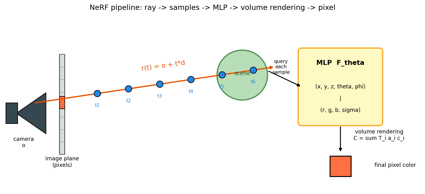
NeRF pipeline: a camera ray r(t) = o + t·d passes through a pixel into the scene; sample points along the ray are fed to the MLP F_Θ, which returns (r, g, b, σ) each; volume rendering composites them into the final pixel color. বাংলা: NeRF pipeline — camera থেকে pixel ভেদ করে ray r(t) = o + t·d scene-এ ঢোকে; ray-এর উপর sample point-গুলো MLP F_Θ-কে দেওয়া হয়, প্রতিটার জন্য (r, g, b, σ) ফেরত আসে; volume rendering সেগুলো মিশিয়ে pixel-এর চূড়ান্ত রঙ বানায়।
Every piece of the chapter sits in this one picture: ray (§4.2), samples (§4.4), the 5-D→4-D function (§4.1), compositing (§4.4–4.6). If you can redraw this from memory, you can answer all five trial-exam statements.
বাংলা: পুরো chapter এই এক ছবিতে: ray, sample, 5-D→4-D function, compositing। স্মৃতি থেকে এটা আঁকতে পারলে trial exam-এর পাঁচটা T/F-ই আপনার।
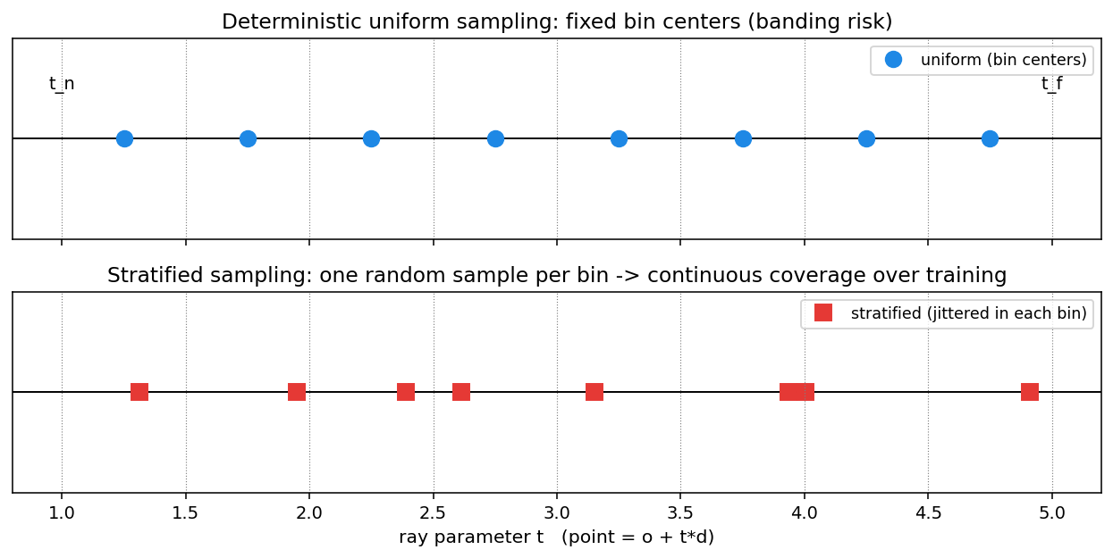
Top: deterministic bin centers — the same depths are queried every time (banding risk, fixed resolution). Bottom: stratified sampling — one uniformly random sample inside each bin, so over many training iterations the network is queried at continuously varying depths. বাংলা: উপরে — প্রতিবার একই নির্দিষ্ট গভীরতায় sample (banding-এর ঝুঁকি, resolution আটকে যায়)। নিচে — stratified sampling: প্রতিটা bin-এর ভেতরে এলোমেলো একটা জায়গায় sample, ফলে বহু iteration মিলিয়ে network-কে অবিরত ভিন্ন ভিন্ন গভীরতায় প্রশ্ন করা হয় — continuous representation শেখে।
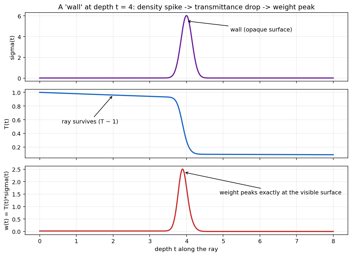
A synthetic 1-D density profile with a "wall" at depth t = 4. Top: σ(t) spikes at the wall. Middle: transmittance T(t) ≈ 1 before the wall, collapses to ≈ 0 across it. Bottom: the weight w(t) = T(t)·σ(t) is a sharp peak exactly at the visible surface. বাংলা: t = 4-এ একটা "দেয়াল"-ওয়ালা কৃত্রিম 1-D density profile। উপরে: দেয়ালে σ(t)-এর স্পাইক। মাঝে: transmittance T(t) দেয়ালের আগে ≈ 1, দেয়াল পেরোতেই ≈ 0। নিচে: weight w(t) = T(t)·σ(t) ঠিক দৃশ্যমান surface-এই তীক্ষ্ণ চূড়া — রঙ আর depth দুটোই এখান থেকে আসে।
This is the picture to recall when asked "why does NeRF see surfaces?": the product of "still alive" (T) and "stops here" (σ) is nonzero only in a thin shell at the first opaque thing the ray meets.
বাংলা: "NeRF surface দেখে কেন?" — কারণ "এখনো বেঁচে আছি" (T) আর "এখানে থামছি" (σ)-এর গুণফল কেবল প্রথম অস্বচ্ছ জিনিসটার পাতলা খোলসে শূন্য নয়।
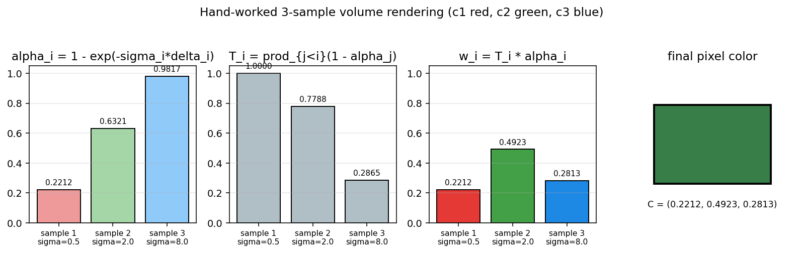
The §4.5 computation visualized: per-sample opacities α_i, running transmittances T_i, weights w_i = T_i·α_i, and the final composited color C = (0.2212, 0.4923, 0.2813). The nearly opaque blue sample 3 receives less weight than the green sample 2 in front of it. বাংলা: §4.5-এর হিসাবটাই ছবি হয়ে: প্রতিটা sample-এর α_i, চলমান T_i, ওজন w_i = T_i·α_i, আর চূড়ান্ত রঙ C = (0.2212, 0.4923, 0.2813)। প্রায়-অস্বচ্ছ নীল sample 3 তার সামনের সবুজ sample 2-এর চেয়ে কম ওজন পায় — সামনে দাঁড়ানোর সুবিধা।
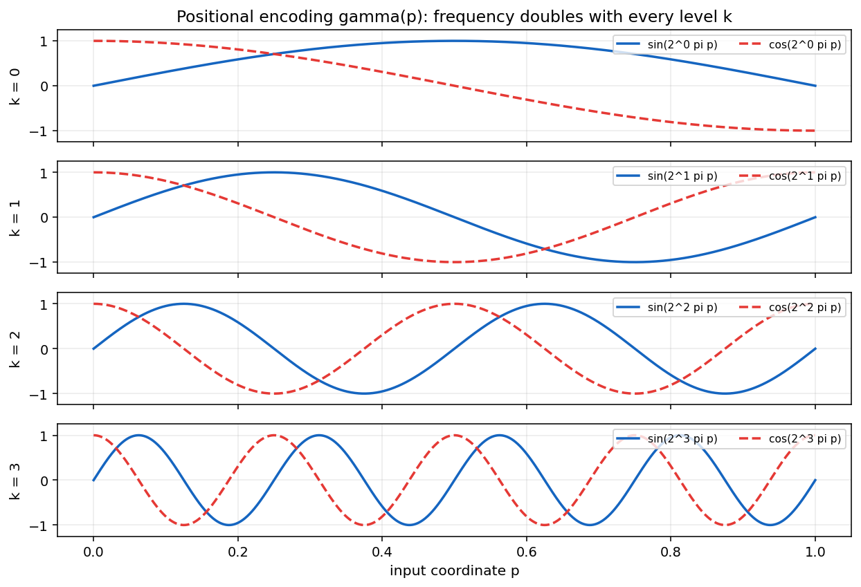
The sin/cos pairs of γ(p) for k = 0…3: each level doubles the frequency. A scene detail that oscillates fast in p is a slow, linearly readable pattern in the high-k coordinates. বাংলা: γ(p)-এর sin/cos জোড়া, k = 0…3 — প্রতি ধাপে frequency দ্বিগুণ। p-তে যে detail দ্রুত দোলে, উঁচু k-এর অক্ষে সেটা ধীর, সরলরৈখিকভাবে পড়া-যায় এমন প্যাটার্ন — MLP-কে আর high frequency বানাতে হয় না।
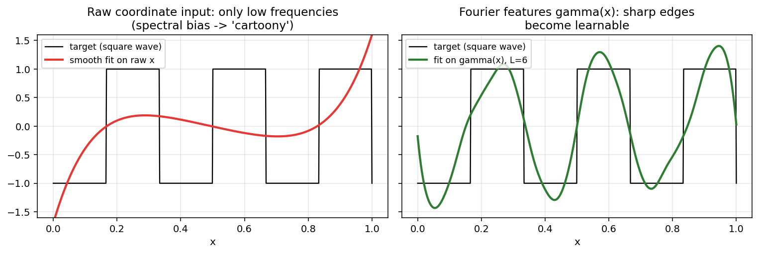
Fitting a square wave. Left: a smooth low-order model on the raw coordinate (the behavior of an MLP without encoding) captures only the low-frequency trend — the "cartoony" failure. Right: the same linear fitting on Fourier features γ(x) with L = 6 reproduces the sharp steps. বাংলা: একটা square wave-এ fit করার চেষ্টা। বাঁয়ে: raw coordinate-এর উপর মসৃণ low-order model (encoding-ছাড়া MLP-র আচরণ) শুধু low-frequency গড়টা ধরে — সেই "cartoon" ব্যর্থতা। ডানে: একই সরল fitting, কিন্তু Fourier feature γ(x) (L = 6)-এর উপর — ধারালো ধাপগুলো হুবহু ফোটে। ভিত্তিফাংশন বদলালেই ক্ষমতা বদলায়।
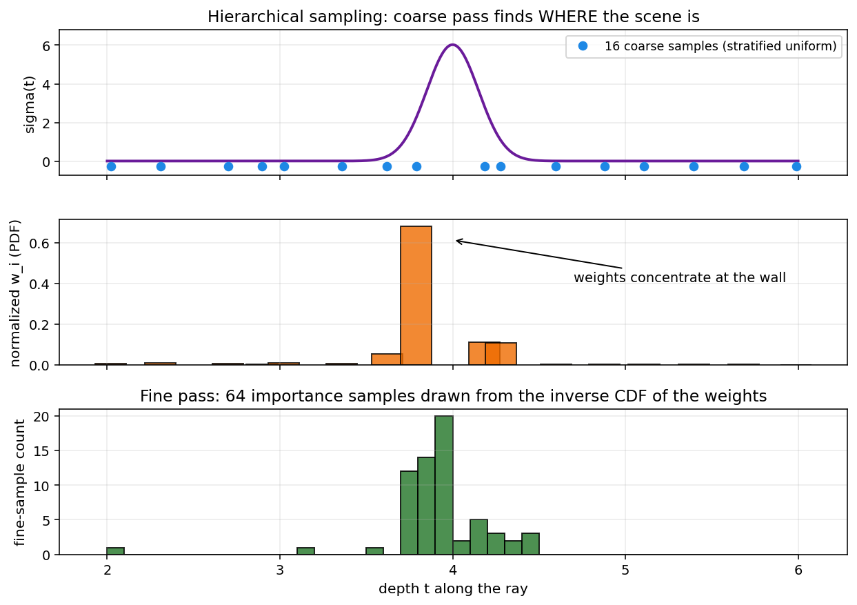
Top: 16 stratified coarse samples along a ray whose density has a wall at t = 4. Middle: the normalized coarse weights form a PDF concentrated at the wall. Bottom: 64 fine samples drawn via the inverse CDF pile up exactly at the surface. বাংলা: উপরে: t = 4-এ দেয়াল-ওয়ালা ray-তে ১৬টা stratified coarse sample। মাঝে: normalize-করা coarse weight-গুলো দেয়ালে কেন্দ্রীভূত একটা PDF। নিচে: inverse CDF দিয়ে টানা ৬৪টা fine sample ঠিক surface-এই স্তূপ — ফাঁকা জায়গায় আর একটাও compute নষ্ট হয় না।
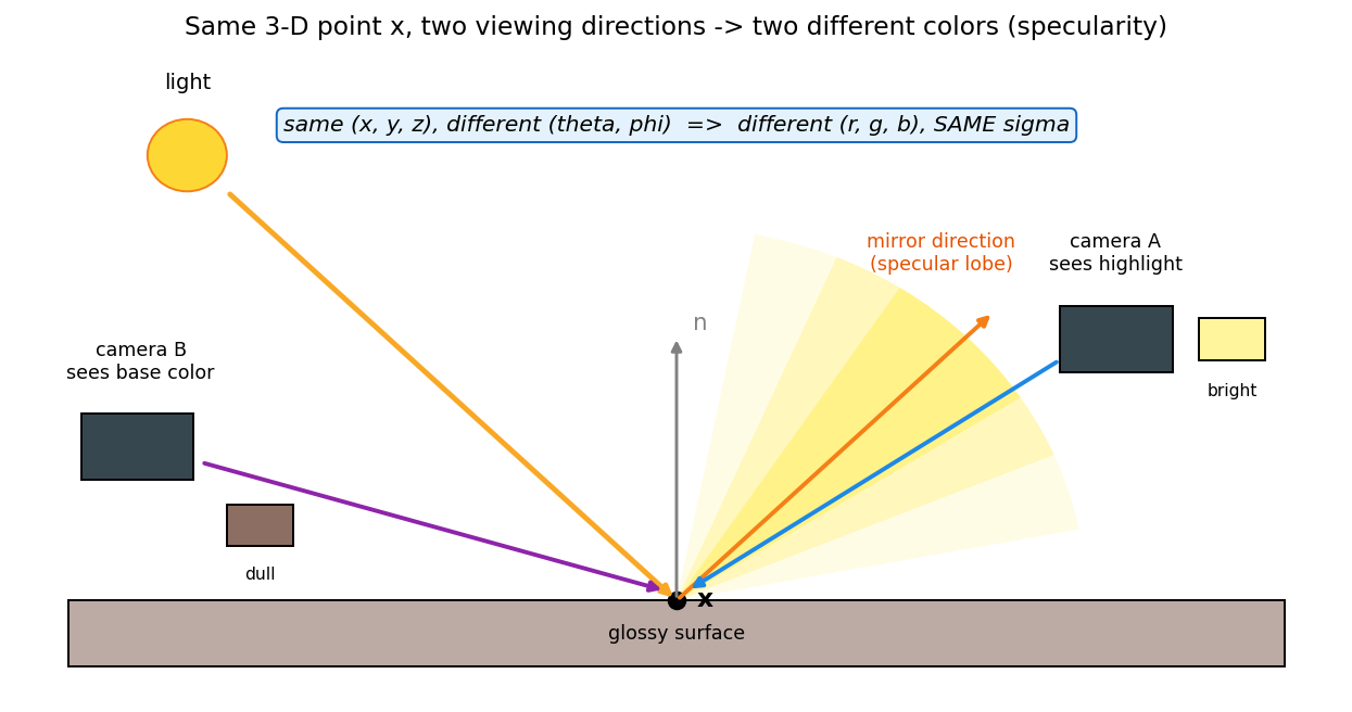
The same surface point x answers differently to two cameras: camera A sits inside the specular lobe (mirror direction of the light) and sees a bright highlight; camera B outside the lobe sees the dull base color. The direction input (θ, φ) changes (r, g, b) — but σ stays identical. বাংলা: একই surface point x দুই camera-কে দুই উত্তর দেয়: camera A আলোর mirror direction-এর specular lobe-এর ভেতরে — উজ্জ্বল highlight দেখে; camera B lobe-এর বাইরে — ম্লান base রঙ দেখে। Direction input (θ, φ) বদলালে (r, g, b) বদলায় — কিন্তু σ একদম একই থাকে। এটাই 5-D input-এর কারণ আর "σ direction-নিরপেক্ষ" নীতির ছবি।
Gallery index — which figure answers which exam question¶
| Figure | Formula it draws | Exam question it answers |
|---|---|---|
ch11_nerf_overview |
\(F_\Theta (x,y,z,\theta ,\phi ) \to (r,g,b,\sigma )\) + \(r(t) = o + t\cdot d\) | "Sketch/describe the NeRF pipeline" — and all five trial T/F at once |
ch11_ray_sampling |
stratified \(t_{i}\), one per bin | "Why jitter instead of fixed bin centers?" (Mock B5) |
ch11_transmittance_weights |
\(T(t) = e^(-\int \sigma )\), \(w = T\cdot \sigma\) | "Why does the weight peak at the first surface?" (Mock B3) |
ch11_three_sample_example |
\(\alpha _{i}, T_{i}, w_{i}, \hat{C} = \Sigma w_{i} c_{i}\) | every hand-computation question (Mock C1, C4) |
ch11_positional_encoding |
\(\gamma (p)\), frequencies ×2 per level | "Write down γ(p); count dimensions" (Mock C2, C3) |
ch11_spectral_bias |
raw-coordinate fit vs Fourier-feature fit | "Why cartoony without γ?" (Mock A4) |
ch11_hierarchical_sampling |
weights → PDF → CDF → fine samples | "Explain coarse-to-fine importance sampling" (Mock C5, D2b) |
ch11_view_dependent_color |
c(x, d) varies, \(\sigma (x)\) fixed |
"Why may color depend on direction but not density?" (Mock B4) |
বাংলা: এই ছকটা revision-এর শেষ দিনের জন্য: প্রতিটা ছবি = একটা সূত্র = একটা সম্ভাব্য প্রশ্ন। ছবিগুলো চোখ বুজে আঁকতে পারা মানে সূত্রগুলোও মুখস্থ — আর তাতেই Q10-এর ১০ নম্বর।
§6 Algorithms & Code¶
6.1 NeRF rendering — pseudocode¶
For each pixel:
  1. Build the camera ray: origin o, direction d        (pose + intrinsics, Ch. 10)
  2. Stratified-sample N_c = 64 coarse points t_i in [t_n, t_f]
  3. Query F_Θ^coarse at each (γ(r(t_i)), γ(d)) → (c_i, σ_i)
  4. δ_i = t_{i+1} − t_i;  α_i = 1 − exp(−σ_i δ_i);  T_i = Π_{j<i}(1 − α_j);  w_i = T_i α_i
  5. Coarse color Ĉ_c = Σ w_i c_i  (and expected depth D = Σ w_i t_i)
  6. Normalize w → PDF → CDF; inverse-transform-draw N_f = 128 fine points
  7. Query F_Θ^fine on the union (64 + 128 = 192 points); composite → final Ĉ_f
বাংলা: ধাপগুলো মুখস্থ নয় — বুঝে রাখুন: ray বানাও (Ch. 10-এর pose লাগবেই), মোটা sample, network-কে প্রশ্ন, α/T/w-এর হিসাব (§4.4), রঙ+depth, weight থেকে PDF→CDF→fine sample (§4.10), দুই set মিলিয়ে চূড়ান্ত রঙ। পরীক্ষায় কোনো এক ধাপ ফাঁকা-ভরাট আসতে পারে।
6.2 Training loop — pseudocode¶
Repeat until converged (~10⁵–10⁶ iterations):
  1. Sample a random batch of rays across ALL training images (each ray: o, d, C_gt — 9 numbers)
  2. Render Ĉ_c and Ĉ_f for every ray (procedure 6.1)
  3. L = Σ ‖Ĉ_c − C_gt‖² + ‖Ĉ_f − C_gt‖²
  4. Adam step on both networks (everything is differentiable)
বাংলা: Training মানে: এলোমেলো ray-এর batch → দুই network দিয়েই render → ফটোর সাথে squared error → Adam। লক্ষ করুন coarse loss-ও আছে — সে ভালো না হলে fine sampling-ই ভুল জায়গায় পড়বে।
6.3 Positional encoding in NumPy (worth writing by hand once)¶
import numpy as np

def pos_enc(p, L):
    """p: (..., D) array in ~[-1, 1]. Returns (..., 2*L*D) encoding (paper version)."""
    out = []
    for k in range(L):
        out.append(np.sin(2**k * np.pi * p))
        out.append(np.cos(2**k * np.pi * p))
    return np.concatenate(out, axis=-1)

print(pos_enc(np.array([0.25]), L=2))   # [0.7071 0.7071 1.     0.    ] — (sin πp, cos πp, sin 2πp, cos 2πp)
# 3-D position, L=10 → 60 dims; direction, L=4 → 24 dims (+3 each if raw input appended)
বাংলা: নিজে একবার লিখুন — তাহলেই dimension-গোনা প্রশ্নে আর ভুল হবে না: প্রতি স্কেলারে 2Lটা সংখ্যা, 3-vector-এ 6Lটা।
6.4 Tiny NeRF MLP (PyTorch, architecture-faithful)¶
import torch, torch.nn as nn

class TinyNeRF(nn.Module):
    def __init__(self, L_pos=10, L_dir=4, hidden=128):
        super().__init__()
        self.L_pos, self.L_dir = L_pos, L_dir
        in_pos = 3 + 3*2*L_pos          # 63: raw xyz + encoding
        in_dir = 3 + 3*2*L_dir          # 27: raw dir + encoding
        self.body = nn.Sequential(
            nn.Linear(in_pos, hidden), nn.ReLU(),
            nn.Linear(hidden, hidden), nn.ReLU(),
            nn.Linear(hidden, hidden), nn.ReLU())
        self.sigma_head = nn.Linear(hidden, 1)        # density: BEFORE direction joins
        self.feat = nn.Linear(hidden, hidden)
        self.color_head = nn.Sequential(              # direction enters only here
            nn.Linear(hidden + in_dir, hidden // 2), nn.ReLU(),
            nn.Linear(hidden // 2, 3), nn.Sigmoid())

    @staticmethod
    def enc(x, L):
        out = [x]
        for k in range(L):
            out += [torch.sin(2**k * torch.pi * x), torch.cos(2**k * torch.pi * x)]
        return torch.cat(out, dim=-1)

    def forward(self, pos, view_dir):
        h = self.body(self.enc(pos, self.L_pos))
        sigma = torch.relu(self.sigma_head(h)).squeeze(-1)   # σ ≥ 0, view-independent
        rgb = self.color_head(torch.cat([self.feat(h),
                                         self.enc(view_dir, self.L_dir)], dim=-1))
        return sigma, rgb
বাংলা: Code-এ স্থাপত্যের দুটো নীতি দেখুন: sigma_head বসে direction যোগ হওয়ার আগে (geometry view-নিরপেক্ষ), আর color_head-এ direction ঢোকে শেষে (penultimate layer)। ReLU দিয়ে σ ≥ 0, sigmoid দিয়ে রঙ [0,1]-এ।
6.5 Differentiable volume rendering of one ray (PyTorch)¶
def render_ray(model, o, d, near, far, N=64):
    t = torch.linspace(near, far, N)
    pts = o + t[:, None] * d                      # (N, 3) sample positions
    sigma, rgb = model(pts, d.expand_as(pts))     # query the field
    delta = torch.cat([t[1:] - t[:-1],
                       torch.tensor([1e10])])     # last segment "infinite"
    alpha = 1.0 - torch.exp(-sigma * delta)                       # α_i = 1 − e^(−σδ)
    trans = torch.cumprod(torch.cat([torch.ones(1),
                                     1.0 - alpha + 1e-10]), 0)[:-1]   # T_i = Π(1−α_j), j<i
    w = trans * alpha                                              # w_i = T_i α_i
    color = (w[:, None] * rgb).sum(0)             # Ĉ = Σ w_i c_i
    depth = (w * t).sum(0)                        # D = Σ w_i t_i
    return color, depth, w
Implementation notes: the shifted cumprod (prepend a 1, drop the last entry) implements "product over j strictly less than i"; the 1e10 final delta makes the last sample absorb all remaining light if it is dense; the 1e-10 avoids a zero in the product chain killing gradients.
বাংলা: তিনটা সূক্ষ্মতা খেয়াল করুন: (১) cumprod-এর আগে 1 জুড়ে শেষেরটা ফেলে দেওয়া — এতেই "j < i" (strictly less) হয়; (২) শেষ δ = 10¹⁰ — শেষ sample ঘন হলে বাকি সব আলো সে-ই নেবে; (৩) 1e-10 — গুণফলের চেইনে শূন্য এলে gradient মরে যায়, তার বীমা। মুখস্থ লাইন: w = trans * alpha, color = Σ w·rgb, \(depth = \Sigma w\cdot t\)।
6.6 Optional: mesh extraction afterwards (marching cubes)¶
1. Evaluate σ on a dense 3-D grid (the network is queried like a voxel volume).
2. Threshold (e.g. σ > 50) → occupancy.
3. Marching cubes → triangle mesh.
Not part of NeRF's rendering — exists only to interface with classic pipelines. (This is why trial statement "NeRFs explicitly reconstruct a mesh before rendering" is FALSE.)
বাংলা: Mesh চাইলে training-এর পরে σ-কে grid-এ মেপে marching cubes চালানো যায় — কিন্তু এটা NeRF-এর rendering-এর অংশ নয়। তাই "NeRF rendering-এর আগে mesh বানায়" — FALSE।
6.7 The spectral-bias toy experiment — 2-D image regression (lecture demo, in code)¶
The single most convincing experiment in the whole chapter, reproduced in ~25 lines: train one MLP to memorize one image as a function \((u, v) \to (r, g, b)\), once with and once without positional encoding.
import torch, torch.nn as nn

class CoordMLP(nn.Module):
    """Memorize ONE image: (u, v) → (r, g, b). The lecture's spectral-bias demo."""
    def __init__(self, with_pe=True, L=10):
        super().__init__()
        self.with_pe, self.L = with_pe, L
        in_dim = 2 + 2 * 2 * L if with_pe else 2     # 2 coords × 2 fns × L levels (+ raw)
        self.net = nn.Sequential(
            nn.Linear(in_dim, 128), nn.ReLU(),
            nn.Linear(128, 128), nn.ReLU(),
            nn.Linear(128, 3), nn.Sigmoid())

    def forward(self, uv):                            # uv in [-1, 1]^2
        if self.with_pe:
            outs = [uv]
            for k in range(self.L):
                outs += [torch.sin(2**k * torch.pi * uv),
                         torch.cos(2**k * torch.pi * uv)]
            uv = torch.cat(outs, dim=-1)
        return self.net(uv)

# Training sketch: uv grid of all pixel centers, target = the image's RGB values.
# for step in range(2000):
#     loss = ((model(uv) - rgb_gt) ** 2).mean();  loss.backward();  opt.step();  opt.zero_grad()
What you will observe (and should be able to predict in the exam):
with_pe=False: the loss plateaus early; the reconstruction looks like a bilateral-filtered cartoon — smooth color regions, all edges and texture gone. More training does not help: the failure is the spectral bias itself, not under-training.with_pe=True: the loss keeps dropping and the network reproduces every detail of the image.- Sweep
L= 2, 6, 10: detail sharpens with each step, with diminishing returns — the "frequency count is a hyperparameter" point of §2.8.
This 2-D toy is NeRF's situation in miniature: NeRF is the same coordinate-regression idea, just in 3-D, with σ added and a rendering integral between the network and the loss.
বাংলা: পুরো chapter-এর সবচেয়ে বিশ্বাস-জাগানো পরীক্ষাটা নিজে চালান: একটা MLP-কে একটা ছবি মুখস্থ করতে দিন — \((u, v) \to (r, g, b)\) — একবার positional encoding ছাড়া, একবার সহ। ছাড়া: loss আগেই থেমে যায়, ফল bilateral-filter-করা cartoon — ধার আর texture উধাও; বেশি train করলেও সারে না, কারণ রোগটা training-এর নয়, spectral bias-এর। সহ: প্রতিটা খুঁটিনাটি ফিরে আসে। L = 2, 6, 10 ঘুরিয়ে দেখুন — ধাপে ধাপে ধারালো, কিন্তু লাভ ক্রমে কমে। মনে রাখুন: এই 2-D খেলনাটাই ক্ষুদ্রাকারে NeRF — শুধু 3-D, সাথে σ আর loss-এর আগে একটা rendering integral।
§7 Trial-Exam Mapping¶
| Trial Q10 statement | Answer | Where & why |
|---|---|---|
| 1. NeRFs learn a mapping from 3-D coordinates and view direction to color and density. | TRUE | §4.1 — \(F_\Theta (x, y, z, \theta , \phi ) \to (r, g, b, \sigma )\), verbatim |
| 2. NeRFs rely on voxel grids for storing scene geometry. | FALSE | §2.4/§2.5 — the voxel grid is replaced by the MLP; geometry lives implicitly in weights |
| 3. NeRF training requires multiple posed images of a static scene. | TRUE | §2.10/§4.9 — photometric loss vs posed photos; poses from SfM/COLMAP; static for consistency |
| 4. NeRFs explicitly reconstruct a mesh before rendering. | FALSE | §6.6 — rendering is direct ray marching; meshes only via optional post-hoc marching cubes |
| 5. NeRFs use ray marching to accumulate color along sampled points. | TRUE | §4.4 — \(\hat{C} = \Sigma T_{i} \alpha _{i} c_{i}\) over samples along each ray |
বাংলা: পাঁচটা statement-এর প্রত্যেকটার এক-লাইনের যুক্তি মুখস্থ রাখুন; T/F-এ "কেন" জানা থাকলে উল্টো করে বানানো নতুন statement-ও ধরা যায় (যেমন: "σ viewing direction-এর উপর নির্ভর করে" — FALSE; "রঙ করে" — TRUE)।
Extra T/F bank — the statements the examiner could swap in¶
The trial exam's five statements are one draw from a small pool. Cover the answers and test yourself on twelve plausible alternates:
| # | Statement | Answer | One-line why |
|---|---|---|---|
| 1 | The density output σ depends on the viewing direction. | F | σ branches off before the direction enters the MLP — geometry must be view-consistent |
| 2 | The color output can change when only the viewing direction changes. | T | view-dependent radiance — specular highlights move with the camera |
| 3 | NeRF is trained with a depth-supervision loss (e.g. against LiDAR). | F | photometric loss only — \(\Sigma \|\hat{C} - C_{gt}\|^{2}\); no 3-D labels at all |
| 4 | Positional encoding maps each input scalar to 2L sin/cos values at doubling frequencies. | T | \(\gamma (p)\), L = 10 (pos) / 4 (dir) → 60 / 24 dims |
| 5 | Without positional encoding, NeRF renders look cartoonish and lack detail. | T | spectral bias of MLPs on raw coordinates |
| 6 | The fine pass of hierarchical sampling places its samples uniformly along the ray. | F | importance sampling from the coarse weights' CDF — samples cluster at surfaces |
| 7 | The compositing weights w_i along a ray always sum to exactly 1. | F | \(\Sigma w = 1 - T_{N+1} \le 1\); the remainder is the escaping (background) light |
| 8 | A NeRF trained on one scene can render a different scene without retraining. | F | per-scene optimization — the weights are the scene |
| 9 | Camera poses for NeRF training are typically estimated with SfM/COLMAP. | T | Chapter 10's pipeline feeds Chapter 11 |
| 10 | NeRF's compositing is the same alpha compositing used in classic CT/MRI volume rendering. | T | identical \(\Sigma T_{i} \alpha _{i} c_{i}\); only the voxel lookup became an MLP query |
| 11 | The viewing direction is part of the input to the first layer of NeRF's MLP. | F | it is concatenated only at the penultimate layer (shape-radiance fix) |
| 12 | α_i and σ_i are the same quantity in different notation. | F | \(\alpha _{i} = 1 - e^(-\sigma _{i} \delta _{i})\): σ is a rate (unbounded, per length), α a fraction in [0, 1) |
বাংলা: Trial-এর পাঁচটা statement একটা ছোট পুকুর থেকে তোলা পাঁচটা মাছ — পুকুরটাই মুখস্থ করুন। উপরের ১২টা বিকল্পের প্রতিটার "কেন"-সহ উত্তর বলতে পারলে Q10-এ যে সংস্করণই আসুক, ১০ নম্বর আপনার। বিশেষ ফাঁদ তিনটা: σ বনাম α (rate বনাম fraction), ওজনের যোগফল (ঠিক ১ নয়, ≤ ১), আর direction কোথায় ঢোকে (প্রথম layer-এ নয়, penultimate-এ)।
§8 Mock Exam — 20 Questions¶
Work through the questions before reading the solutions. Calculators allowed for Tier C; useful constants: e^(−0.25) ≈ 0.7788, e^(−0.5) ≈ 0.6065, e^(−1) ≈ 0.3679, e^(−1.5) ≈ 0.2231, e^(−4) ≈ 0.0183.
Tier A — Basic (1 point each)¶
A1. Write down the NeRF scene function: all inputs, all outputs, and one sentence on the meaning of σ.
A2. Mark each statement TRUE or FALSE: (a) A NeRF stores the scene in a voxel grid. (b) The color output may depend on the viewing direction. © The density output may depend on the viewing direction. (d) Rendering uses ray marching with alpha compositing. (e) A trained NeRF generalizes to other scenes without retraining.
A3. Define transmittance T(t) — formula and one-sentence physical meaning.
A4. What is positional encoding, and what failure does it prevent? (Two sentences.)
A5. Name two limitations of vanilla NeRF (with the lecture's rough numbers) and one successor method that addresses each.
Tier B — Intuitive (2 points each)¶
B1. A light field needs only 4 inputs (a ray) instead of NeRF's 5. Why did Mildenhall et al. choose the more expensive 5-D volumetric function?
B2. Why does NeRF training require (a) a static scene, (b) known camera poses, and © many views with varied positions? State what goes wrong if each is violated, and where the poses come from in practice.
B3. Explain physically why the weight function \(w(t) = T(t)\cdot \sigma (t)\) peaks exactly at the first visible surface — using the behavior of T and σ before, at, and behind the surface.
B4. Why does it make sense that the same 3-D point can output different colors for two cameras, but never different densities? Give a concrete optical example.
B5. Coarse samples could simply be placed at the fixed centers of N uniform bins. Why does NeRF instead jitter one random sample per bin (stratified sampling)?
Tier C — Harder / Computational (3 points each)¶
C1. A ray has three samples with σ = (1.0, 2.0, 0.5), all δ_i = 0.5, and colors c₁ = (1, 0, 0), c₂ = (0, 1, 0), c₃ = (1, 1, 1). Compute α_i, T_i, w_i, the weight sum, and the final color Ĉ. Verify Σw against 1 − e^(−Σσδ).
C2. Compute the positional encoding γ(p) with L = 2 for (a) p = 0.5 and (b) p = 0.25. (Exact values where possible.)
C3. NeRF uses L = 10 for the position and L = 4 for the direction. (a) How many encoded dimensions does each produce? (b) How many input dimensions in total reach the network if the raw 3-vectors are appended too? © A colleague proposes L = 14 for positions — what trade-off are they making?
C4. Using the weights of the worked example in §4.5 — w = (0.221199, 0.492296, 0.281257) at depths t = (1.0, 1.5, 2.0) — compute the expected depth D = Σ w_i t_i and the normalized depth D / Σ w_i.
C5. A coarse pass yields normalized weights (0.05, 0.10, 0.60, 0.25) on the depth bins [1, 1.5), [1.5, 2), [2, 2.5), [2.5, 3). Build the CDF, then place fine samples for the uniform draws u = 0.40 and u = 0.90 (linear interpolation within the bin). Which bin receives the most fine samples in expectation, and what fraction?
Tier D — Transfer (4 points each)¶
D1. In NeRF's MLP the viewing direction is concatenated only at the penultimate layer, while the position enters at the start (and again via a skip connection). Explain (a) what the shape-radiance ambiguity is, (b) why a "vanilla" MLP receiving the full 5-D input from layer 1 produces floaters and broken geometry, and © why the late-direction architecture pushes the network toward correct, view-consistent geometry while still allowing specular highlights.
D2. (a) Prove that the rendering weights satisfy \(\Sigma _{i} w_{i} = 1 - T_{N+1} \le 1\) and interpret \((w_{1},\ldots ,w_{N}, T_{N+1})\) probabilistically. (b) Explain why drawing fine samples from the normalized weights via the inverse CDF is importance sampling, and what quantity it improves for a fixed sample budget.
D3. Compare NeRF with 3D Gaussian Splatting along: scene representation (implicit vs explicit), rendering algorithm, rendering speed, and training. Then explain the key idea of instant-NGP's hash encoding and why it accelerates training by orders of magnitude.
D4. (a) Why does NeRF degrade badly with very few input views — name the two ambiguities that become unconstrained. (b) Why does it fail with inaccurate camera poses, and which Chapter-10 pipeline provides the poses? © Sketch what happens to the photometric loss landscape when pose noise grows.
D5. (a) Show by unrolling the front-to-back compositing recursion \(C \leftarrow C + T\cdot \alpha _{i}\cdot c_{i}, T \leftarrow T\cdot (1-\alpha _{i})\) for N = 3 that it produces exactly NeRF's quadrature \(\Sigma T_{i} \alpha _{i} c_{i}\). (b) Vanilla NeRF aliases when a far-away object covers less than a pixel. Explain why point-sampled rays cause this and the mip-NeRF idea that fixes it.
Solutions¶
Tier A¶
A1. \(F_\Theta : (x, y, z, \theta , \phi ) \to (r, g, b, \sigma )\). Inputs: 3-D position of the query point plus the viewing direction (two polar angles, or equivalently a unit 3-vector). Outputs: emitted RGB color at that point as seen from that direction, and the volume density σ — the rate (per unit length, σ ≥ 0) at which a ray is absorbed there; "geometry" in NeRF is nothing but regions of high σ.
বাংলা শিক্ষণীয়: এক লাইনে NeRF: "৫ ঢোকে, ৪ বের হয়" — position+direction ঢোকে, রঙ+density বের হয়; σ মানে প্রতি একক দৈর্ঘ্যে ray থামার হার।
A2. (a) FALSE — the MLP replaces the voxel grid; the scene lives in network weights. (b) TRUE — color is view-dependent (specularity). © FALSE — σ is computed before the direction enters the network; geometry must be view-consistent. (d) TRUE — \(\hat{C} = \Sigma T_{i} \alpha _{i} c_{i}\) along each camera ray. (e) FALSE — vanilla NeRF is a per-scene optimization; a new scene needs a new ~3-day training.
বাংলা শিক্ষণীয়: তিনটা না-বোধক ফাঁদ মনে রাখুন: voxel নেই, σ-তে direction নেই, generalization নেই।
A3. \(T(t) = \exp (-\int _{t_{n}}^t \sigma (r(s)) ds)\). It is the fraction of light (equivalently: the probability) that survives the trip from the near bound to depth t without being absorbed; it starts at 1 and is monotonically non-increasing along the ray.
বাংলা শিক্ষণীয়: T = "এ পর্যন্ত বেঁচে আসার সম্ভাবনা" — শুরুতে ১, পথে শুধুই কমে।
A4. Positional encoding maps each input scalar p to sin/cos pairs at exponentially growing frequencies, \(\gamma (p) = (\sin (2^{0}\pi p), \cos (2^{0}\pi p), \ldots , \sin (2^(L-1)\pi p), \cos (2^(L-1)\pi p))\), before the MLP sees it. It prevents the spectral-bias failure: an MLP on raw low-dimensional coordinates learns only a low-frequency, "cartoony" version of the scene and misses fine detail.
বাংলা শিক্ষণীয়: γ না দিলে NeRF = cartoon; γ দিলে MLP রেডিমেড frequency-গুলো শুধু মেশায়।
A5. Limitations: (1) training ≈ 3 days per scene on a 2080 Ti, rendering 1–2 min/frame — addressed by instant-NGP (hash-grid features + tiny MLP → minutes of training) and by 3D Gaussian Splatting (rasterization → real-time rendering); (2) only static, bounded scenes with per-scene optimization — addressed by NeRF++ (foreground/background split for unbounded scenes) and NeRF in the Wild (static + transient decomposition for tourist photos). (Any two limitations with matching successors earn full marks.)
বাংলা শিক্ষণীয়: সংখ্যাসহ বলুন: ৩ দিন training, ১–২ মিনিট/frame — আর প্রতিকারের নাম জুড়ে দিন।
Tier B¶
B1. Because of smoothness. The 4-D light field maps rays to colors, and adjacent rays can hit entirely different objects (one grazes a silhouette edge, its neighbor misses) — the function is riddled with discontinuities, which small networks approximate poorly. The 5-D volumetric field (density and color in space) varies smoothly almost everywhere, so a compact MLP can represent it; the sharpness in final images is re-created by the rendering integral, not by the network having to learn discontinuities. Bonus symmetry: in free space radiance is constant along rays, so the 5-D field also contains redundancy — but redundancy is cheap, discontinuity is expensive.
বাংলা শিক্ষণীয়: Network মসৃণ জিনিস শিখতে ভালোবাসে — 4-D light field ধারালো-ফাটলে ভরা, 5-D ঘনত্ব-ক্ষেত্র মসৃণ; তাই এক মাত্রা "বেশি খরচ" করেও 5-D জেতে।
B2. (a) Static scene: supervision is multi-view consistency — if the object moves between photos, the same 3-D point is taught contradictory colors/occupancy and the model blurs or ghosts. (b) Known poses: rays are built from pose + intrinsics; wrong poses send rays through wrong pixels, so the same point receives inconsistent colors → mush. Poses come from SfM/COLMAP (Chapter 10) — feature matching, triangulation, bundle adjustment. © Many varied views: geometry is never supervised directly; only parallax across views disambiguates depth. Few/concentrated views leave the shape-radiance and near-field ambiguities unconstrained → floaters and fake geometry that only look right from the training positions. (Lecture's ideal bound: < 1 px parallax between neighboring views — practically unreachable, hence priors and encodings.)
বাংলা শিক্ষণীয়: NeRF-এর একমাত্র শিক্ষক হলো "অনেক view-এর মিল"; scene নড়লে, pose ভুল হলে বা view কম হলে সেই শিক্ষকই অন্ধ।
B3. Before the surface: σ ≈ 0 (empty air), so w = T·σ ≈ 0 even though T ≈ 1 — nothing there to emit. At the surface: T is still ≈ 1 (the light has survived the empty stretch) and σ spikes — both factors are large, so w peaks. Behind the surface: σ may be huge inside the object, but T has collapsed to ≈ 0 because the surface absorbed the ray — so w ≈ 0 again. The product is nonzero only in the thin shell where "still visible" and "something is here" overlap: that is precisely the visible surface, which is why both the color and the expected depth come from there.
বাংলা শিক্ষণীয়: আগে — জিনিস নেই (σ=0); পরে — দেখা যায় না (T=0); ঠিক surface-এ দুটোই বড় — তাই ওজনের চূড়া সেখানেই।
B4. Different colors per direction model view-dependent appearance: a glossy teapot shows a bright specular highlight to a camera sitting near the light's mirror direction, and only its dull base color to a camera elsewhere — same point, two honest colors (figure §5, last image). But density is occupancy: whether matter exists at a point cannot depend on who is looking. If σ were view-dependent, a wall could exist for camera A and vanish for camera B — "geometry" would be inconsistent and novel views would fall apart. Hence the architecture computes σ before the direction is even visible to the network.
বাংলা শিক্ষণীয়: রঙ হলো "কেমন দেখায়" (দিকভেদে বদলায়), σ হলো "আছে কি নেই" (দিকের প্রশ্নই নেই)।
B5. Fixed bin centers query the same N depths for every ray, every iteration. Two problems: (1) the network is only ever supervised at a discrete comb of depths — between them it can do anything (the representation effectively becomes a fixed-resolution grid, and regular structure invites banding/aliasing artifacts aligned with the comb); (2) thin structures sitting between two centers are never sampled and vanish. Stratified sampling keeps the bins (guaranteeing coverage of the whole [t_n, t_f] range — no clumping) but jitters the position inside each bin per iteration, so over training the network is queried at a continuum of depths: a genuinely continuous representation, unbiased quadrature, no banding.
বাংলা শিক্ষণীয়: নির্দিষ্ট চিরুনি-দাঁতে প্রশ্ন করলে network চিরুনিই শেখে; bin রেখে ভেতরে ঝাঁকালে — coverage-ও থাকে, continuity-ও আসে।
Tier C¶
C1. Opacities, with δ = 0.5 everywhere:
Transmittances:
Weights:
w₁ = 1·0.393469        = 0.393469
w₂ = 0.606531·0.632121 = 0.383400
w₃ = 0.223130·0.221199 = 0.049356
Σw = 0.826226 ;  check: 1 − e^(−(0.5+1.0+0.25)) = 1 − e^(−1.75) = 1 − 0.173774 = 0.826226 ✓
Final color:
A dark yellow-orange: the white sample at the back barely matters because only e^(−1.5) ≈ 22% of the light ever reaches it, and it is thin (α₃ ≈ 0.22) on top of that. About 17.4% of the ray escapes (would show background).
বাংলা শিক্ষণীয়: ছক ধরে এগোন — α (প্রতিটা টুকরোর ফাঁদ), T (সামনেরগুলোর ছাড়পত্রের গুণফল), w = T·α, যাচাই Σw = 1 − e^(−Σσδ), শেষে Σw·c। যাচাইয়ের লাইনটাই আপনার ভুল ধরার জাল।
C2. (a) \(\gamma (0.5) = (\sin (\pi /2), \cos (\pi /2), \sin (\pi ), \cos (\pi )) = (1, 0, 0, -1)\) — exact. (b) \(\gamma (0.25) = (\sin (\pi /4), \cos (\pi /4), \sin (\pi /2), \cos (\pi /2)) = (\sqrt{2}/2, \sqrt{2}/2, 1, 0) \approx (0.7071, 0.7071, 1, 0)\). Note the structure: level k = 0 oscillates once over [−1, 1]; level k = 1 twice as fast — that is the "frequency doubling per level."
বাংলা শিক্ষণীয়: L=2 মানে মাত্র চারটা সংখ্যা: (sin πp, cos πp, sin 2πp, cos 2πp) — কোণগুলো ডিগ্রিতে ভাবলে (45°, 90° ইত্যাদি) হিসাব মুখেই হয়।
C3. (a) Position: 3 × 2 × 10 = 60 dims; direction: 3 × 2 × 4 = 24 dims. (b) With raw inputs appended: 60 + 3 = 63 and 24 + 3 = 27; the 63 enter at the first layer, the 27 join at the penultimate layer (they are not concatenated at the input!). © L = 14 gives 3·2·14 = 84 position dims: the network can express even higher frequencies → sharper detail, but with diminishing returns, more parameters/compute, and a growing risk of fitting high-frequency noise (and of aliasing where views are sparse). Frequency count is a genuine hyperparameter — the lecture's "too few = cartoony, more = better but it saturates."
বাংলা শিক্ষণীয়: গোনার সূত্র এক লাইনে: মাত্রা = (vector-এর দৈর্ঘ্য 3) × (sin, cos = 2) × L; আর মনে রাখুন — 63 ঢোকে শুরুতে, 27 ঢোকে penultimate layer-এ।
C4.
D = 0.221199·1.0 + 0.492296·1.5 + 0.281257·2.0
  = 0.221199 + 0.738444 + 0.562515 = 1.522158
D_normalized = 1.522158 / 0.994752 = 1.530187
The expected depth (≈ 1.52–1.53) sits between the fog samples and the back surface — a reminder that expected depth is a mean, which can land "between" surfaces for semi-transparent stacks; the threshold variant (depth where T ≤ 0.01) would report a value at the last sample instead.
বাংলা শিক্ষণীয়: Expected depth হলো ওজন-করা গড় — আধা-স্বচ্ছ দৃশ্যে সে দুই surface-এর মাঝে পড়তে পারে; "৯৯% আলো আটকানোর" threshold-পদ্ধতি তখন অন্য উত্তর দেয়, দুটোই জায়েজ।
C5. CDF: F = (0.05, 0.15, 0.75, 1.00).
u = 0.40: 0.15 < 0.40 ≤ 0.75 → bin 3 = [2.0, 2.5)
   t = 2.0 + (0.40 − 0.15)/0.60 · 0.5 = 2.0 + 0.208333 = 2.208333
u = 0.90: 0.75 < 0.90 ≤ 1.00 → bin 4 = [2.5, 3.0)
   t = 2.5 + (0.90 − 0.75)/0.25 · 0.5 = 2.5 + 0.30 = 2.80
Bin 3 receives the most fine samples in expectation: its weight is 0.60, so 60% of all draws land there — the importance-sampling concentration at the surface.
বাংলা শিক্ষণীয়: CDF বানিয়ে দেখুন u কার ঘরে পড়ে — বড়-weight-এর bin-এর "ঘর" লম্বা, তাই sample সেখানেই জমে; ভেতরের অবস্থান = (u − F_আগের)/ŵ_bin ভগ্নাংশ ধরে linear interpolation।
Tier D¶
D1. (a) Shape-radiance ambiguity: the training loss only constrains the images; a wrong shape (wrong σ field) can still reproduce all training photos exactly if the color function compensates with strong view dependence — e.g. density smeared in front of the true surface whose colors are tuned per-direction so that each training camera sees the right picture. With finite views, infinitely many (shape, radiance) pairs explain the data; the network knows no physics, so all are equally "correct" to it. The near-field ambiguity is the worst case: regions seen by few cameras can host arbitrary floaters. (b) A vanilla MLP with the 5-D input from layer 1 has its full depth and width available to model view-dependent color, so the compensation in (a) is easy — it happily "explains away" bad geometry; the lecture's comparison shows lost detail and weird floating structure next to the skull. Between cameras nothing forces correctness — it only reproduces appearance at the training views. © Entering the direction at the penultimate layer leaves only 1–2 nonlinearities of view-dependent capacity: enough to add a low-dimensional specular lobe on top of a feature vector, far too little to encode "a different fake image per viewpoint." The first 8 layers must therefore explain all views with one view-independent representation — effectively a diffuse-world assumption — which is only possible if the geometry is (approximately) right. Specular highlights survive because they are a small, smooth directional correction. The same logic explains why heavily reflective/mirror scenes still break NeRF: there the true appearance is not a small directional correction.
বাংলা শিক্ষণীয়: মূল বাক্য: "ভুল আকৃতি + চালাক view-dependent রঙ = নিখুঁত training ছবি" — এই ফাঁকিটা বন্ধ করতেই direction-কে দেরিতে ঢোকানো হয়, যাতে নকল করার ক্ষমতাই (capacity) না থাকে; geometry ঠিক হলে তবেই সব view মেলে।
D2. (a) Write each weight as a telescoping difference: \(w_{i} = T_{i} \alpha _{i} = T_{i} (1 - (1-\alpha _{i})) = T_{i} - T_{i}(1-\alpha _{i}) = T_{i} - T_{i+1}\). Summing: \(\Sigma w_{i} = T_{1} - T_{N+1} = 1 - T_{N+1}\), and since \(T_{N+1} = \Pi (1-\alpha _{i}) \in [0,1]\), we get \(\Sigma w_{i} \le 1\), with equality iff some sample is fully opaque (or densities diverge). Probabilistically, define the discrete event "the ray terminates at sample i" with probability \(w_{i}\) and "the ray escapes through the far bound" with probability \(T_{N+1}\): these N+1 numbers are nonnegative and sum to 1 — a complete probability distribution. The rendered color is then the expectation E[c] under this distribution (with the background color attached to the escape event). (b) The fine pass must estimate an integral whose integrand \(T\cdot \sigma \cdot c\) is nearly zero almost everywhere and large in a thin shell. Uniform sampling wastes nearly all evaluations on the zero region; importance sampling draws from a density proportional to the (coarse estimate of the) integrand's magnitude — the normalized weights — via the inverse CDF. For a fixed budget of MLP evaluations this minimizes the variance of the Monte-Carlo/quadrature estimate (it is optimal when the proposal matches the integrand), i.e. sharper surfaces and less noise for the same compute. The coarse network is kept trained (its own loss term) precisely so this proposal stays accurate.
বাংলা শিক্ষণীয়: প্রমাণের চাবি: \(w_{i} = T_{i} - T_{i+1}\) — telescoping-এ সব কেটে \(1 - T_{N+1}\); অর্থ: ওজনগুলো আসলে "কোথায় থামল ray"-এর probability। আর fine sampling মানে সেই probability থেকেই sample টানা — যেখানে কাজ, সেখানেই খরচ; একই বাজেটে কম noise।
D3. Representation: NeRF — implicit: the scene is the weight vector of an MLP; querying anything costs a forward pass; memory is tiny (MBs) and resolution-free. 3DGS — explicit: millions of 3-D Gaussians, each carrying position, anisotropic covariance (shape/orientation), opacity, and view-dependent color (spherical-harmonics coefficients); memory is larger but access is direct. Rendering: NeRF — ray marching: ~hundreds of MLP queries per pixel, then \(\Sigma T_{i} \alpha _{i} c_{i}\). 3DGS — no marching: project (splat) each Gaussian to the screen, sort by depth, and alpha-composite the few splats covering each pixel with the same front-to-back \(\Sigma T \alpha c\) formula — a rasterization pipeline that GPUs eat for breakfast. Speed: NeRF ≈ 1–2 min/frame (vanilla); 3DGS ≥ 30–100+ FPS (real-time). Training: NeRF ~days (vanilla; instant-NGP reduces it to minutes); 3DGS typically tens of minutes, starting from the SfM/COLMAP point cloud, with adaptive densification (splitting/cloning Gaussians where the error is large). Both need posed images from SfM. Instant-NGP's hash encoding: instead of computing 60 sin/cos features and pushing them through 8×256 layers, keep multiresolution grids of trainable feature vectors; a 3-D point is hashed to table entries at each resolution, the looked-up features are interpolated, concatenated, and passed to a tiny (e.g. 2-layer) MLP. Why it is fast: the heavy lifting moves from deep matrix multiplies into O(1) memory lookups; gradients update only the few touched table entries (sparse, local updates instead of every weight); collisions in the hash table are simply tolerated — the training gradients are dominated by the points that matter (high density/visibility), so the table allocates its capacity adaptively without any explicit collision handling. Result: NeRF-quality scenes trained in seconds-to-minutes.
বাংলা শিক্ষণীয়: তুলনার কঙ্কাল: implicit-MLP-raymarch-ধীর (NeRF) বনাম explicit-Gaussian-rasterize-real-time (3DGS) — compositing সূত্র কিন্তু দুজনেরই \(\Sigma T\alpha c\)। আর instant-NGP-র মন্ত্র: "গণনা নয়, lookup" — শেখা feature hash-table-এ, network ছোট্ট, gradient শুধু ছোঁয়া-লাগা ঘরে।
D4. (a) Geometry is supervised only through multi-view consistency. With few views the shape-radiance ambiguity (wrong shapes + compensating colors fit the data) and the near-field ambiguity (regions covered by only one camera are unconstrained — density "floaters" can hang where only that camera looks) both explode: the optimum is no longer unique, and the network picks some solution that matches the training views but collapses from novel ones. (b) Rays are constructed as \(r(t) = o + t\cdot d\) from each image's pose; with a wrong pose, the ray for a pixel doesn't pass through the 3-D point that actually produced that pixel, so the same scene point gets supervised with colors belonging to other points — systematically inconsistent labels. The model answers with blur (the average of inconsistent colors) and duplicated/ghost geometry. Poses come from the Chapter 10 pipeline: SfM (COLMAP) — SIFT-style feature matching → relative poses → triangulation → bundle adjustment; NeRF is literally a consumer of Chapter 10's output (and modern variants like BARF co-optimize poses during training). © With small pose noise the photometric loss minimum simply becomes shallower and the recovered scene slightly blurry (the model spends density to average out misalignments — like camera shake in a long exposure). As noise grows, the loss landscape develops many bad local minima: the model can lower the loss by creating per-view "explanations" (floaters in front of each camera) rather than one consistent scene — training diverges from any meaningful geometry.
বাংলা শিক্ষণীয়: NeRF-এর ভিত্তি Chapter 10-এর pose — pose-ই ভুল হলে প্রতিটা ray ভুল ঠিকানায় চিঠি দেয়; শিক্ষা অসঙ্গত হয়, ফল ঝাপসা ছবি আর ভূতুড়ে geometry। View কম হলে ambiguity-রা লাগামছাড়া — network "পরীক্ষার প্রশ্ন মুখস্থ" করে, নতুন প্রশ্নে ফেল।
D5. (a) Trace the recursion with \(C_{0} = 0, T_{1} = 1\):
Each accumulated term is exactly \(T_{i} \alpha _{i} c_{i}\) with \(T_{i} = \Pi _{j<i}(1-\alpha _{j})\) — the recursion and the closed-form sum \(\Sigma T_{i} \alpha _{i} c_{i}\) are the same computation, i.e. NeRF's quadrature is front-to-back alpha compositing ("over" operator), and the running T even hands you the per-sample weights for free. (b) A pixel does not correspond to a mathematical line but to a cone: it integrates light over a finite footprint that grows with distance. Vanilla NeRF samples an infinitely thin ray at points, so a distant object whose image is smaller than one pixel is represented by a few arbitrary point samples — tiny camera shifts make the samples hit or miss the structure, producing flicker/jaggies, and the scene is queried at a frequency the pixel grid cannot represent (classic aliasing; cf. Nyquist in §2.4). mip-NeRF renders the cone instead: it divides the cone into conical frustums and replaces γ(point) with an integrated positional encoding — the expected value of the sin/cos features over the frustum's volume (closed-form under a Gaussian approximation of the frustum). High frequencies whose period is smaller than the frustum average themselves to ≈ 0, so far-away (large-footprint) queries automatically see a low-pass, "mip-mapped" version of the scene, while close-ups keep full detail — anti-aliasing built into the encoding, one scale-aware network instead of separate coarse/fine MLPs.
বাংলা শিক্ষণীয়: (a) recursion খুলে লিখলেই দেখা যায় — প্রতিটা ধাপে জমা পড়ে ঠিক \(T_{i} \alpha _{i} c_{i}\); NeRF-এর সূত্র আর চিরাচরিত "over" compositing একই জিনিস। (b) Pixel আসলে রেখা নয়, শঙ্কু (cone) — দূরের জিনিসে শঙ্কুর পা চওড়া; বিন্দু-sample তখন কখনো লাগে কখনো ফসকায় → ঝিকিমিকি/aliasing। mip-NeRF-এর সমাধান: frustum-এর উপর encoding-এর গড় নাও — চওড়া পায়ে উঁচু frequency নিজে নিজেই মুছে যায় (built-in low-pass), কাছে গেলে detail ফেরে।
§9 Cheat Sheet¶
- The function: \(F_\Theta (x, y, z, \theta , \phi ) \to (r, g, b, \sigma )\) — 5 in, 4 out; MLP with 9 layers × 256 channels; σ ≥ 0 is opacity-rate per unit length, view-independent; color view-dependent.
- The ray: \(r(t) = o + t\cdot d\), \(t \in [t_{n}, t_{f}]\); o, d from pose + intrinsics (Ch. 10).
- Continuous rendering: \(C = \int T(t)\cdot \sigma (t)\cdot c(t, d) dt\), \(T(t) = \exp (-\int \sigma ds)\) — T solves \(dT/dt = -\sigma T\) (Beer–Lambert); \(T\cdot \sigma\) = pdf of "ray terminates at t"; C is an expected color.
- Discrete rendering: \(\delta _{i} = t_{i+1}-t_{i}\); \(\alpha _{i} = 1 - e^(-\sigma _{i} \delta _{i})\); \(T_{i} = \Pi _{j<i}(1-\alpha _{j})\); \(w_{i} = T_{i} \alpha _{i}\); \(\hat{C} = \Sigma w_{i} c_{i}\); \(D = \Sigma w_{i} t_{i}\).
- Weight budget: \(w_{i} = T_{i} - T_{i+1}\) ⇒ \(\Sigma w_{i} = 1 - T_{N+1} \le 1\); leftover = background's share; identical to front-to-back "over" compositing.
- Worked numbers to trust your method: σ = (0.5, 2, 8), δ = 0.5: α = (0.2212, 0.6321, 0.9817), T = (1, 0.7788, 0.2865), w = (0.2212, 0.4923, 0.2813), Σw = 0.9948, Ĉ(R,G,B-pure) = (0.2212, 0.4923, 0.2813).
- Positional encoding: \(\gamma (p) = (\sin 2^{0}\pi p, \cos 2^{0}\pi p, \ldots , \sin 2^(L-1)\pi p, \cos 2^(L-1)\pi p)\); cures spectral bias (raw-input MLPs learn low frequencies → cartoony). Dims: pos L=10 → 60 (63 with raw), dir L=4 → 24 (27 with raw). \(\gamma (0.5)|L=2 = (1, 0, 0, -1)\).
- Architecture: σ branch never sees the direction; direction joins at the penultimate layer → blocks shape-radiance ambiguity, allows specularity; skip connection re-injects γ(x).
- Training: \(L = \Sigma \|\hat{C}(r) - C_{gt}(r)\|^{2}\) (coarse + fine), random ray batches; 9 numbers/pixel; needs many posed images of a static scene (poses: SfM/COLMAP); no 3-D supervision.
- Hierarchical sampling: coarse N_c = 64 stratified → weights → PDF → CDF → inverse-transform draw N_f = 128 fine samples → composite the union (≈ 256 MLP queries/pixel).
- Limits: ~3 days training/scene (2080 Ti), 1–2 min/frame, static + bounded, per-scene. NeRF++ (fg/bg split), NeRF-W (static + transient + appearance embeddings), instant-NGP (hash-grid features, minutes), 3DGS (explicit Gaussians, rasterized, real-time), mip-NeRF (cone tracing, integrated PE, anti-aliasing).
- Trial T/F: maps-coords-and-direction-to-color-and-density T · voxel grids F · posed static images T · mesh before rendering F · ray marching T.
বাংলা: শেষ মুহূর্তের সারাংশ — (১) Function: ৫ ঢোকে (position + direction), ৪ বের হয় (রঙ + σ); σ দিক-নিরপেক্ষ, রঙ দিক-নির্ভর। (২) Rendering: ray ধরে sample → \(\alpha = 1 - e^(-\sigma \delta )\) → \(T = \Pi (1-\alpha )\) → \(w = T\alpha\) → রঙ \(\Sigma w c\), depth \(\Sigma w t\); ওজনের যোগফল কখনো ১ ছাড়ায় না (Σw = 1 − T_শেষ), বাকিটা background-এর। (৩) γ ছাড়া cartoon — spectral bias; মাত্রা গোনা: 3×2×L (60/63 আর 24/27)। (৪) Direction ঢোকে penultimate layer-এ — ভুল geometry-কে রঙ দিয়ে ঢাকার ক্ষমতা কেড়ে নেওয়া হয়। (৫) Training: শুধু photometric loss + COLMAP-এর pose + static scene; 3-D supervision নেই। (৬) Hierarchical: coarse ৬৪ → weight-এর CDF → fine ১২৮ — surface-এ sample জমে। (৭) দাম: ৩ দিন/scene, ১–২ মিনিট/frame; প্রতিকার: instant-NGP (hash lookup), 3DGS (rasterize, real-time)।
Common mistakes — the seven classic ways to lose these points¶
- Confusing σ with α. σ is an unbounded rate (per unit length); α = 1 − e^(−σδ) is a fraction in [0, 1). Writing "σ ∈ [0, 1]" or "α = σδ" is an instant red flag (the latter is only the small-σδ approximation).
- Including sample i in its own transmittance. \(T_{i} = \Pi _{j<i}(1 - \alpha _{j})\) — strictly before i. In code: the shifted cumprod (prepend 1, drop last). Including \((1 - \alpha _{i})\) gives the exit transmittance \(T_{i+1}\).
- Claiming Σw_i = 1. It is \(1 - T_{N+1} \le 1\); the leftover is the light that escapes to the background. Use Σw = 1 − e^(−Σσ_jδ_j) as your arithmetic check in every computation question.
- Feeding the view direction too early (or saying it enters at the input). It enters at the penultimate layer; early entry re-opens the shape-radiance ambiguity → floaters.
- Forgetting positional encoding in dimension counts or in "why cartoony?" questions. Counts: 3·2·10 = 60 (pos), 3·2·4 = 24 (dir); 63/27 with raw inputs appended.
- Wrong training requirements. Needed: many photos, static scene, known poses + intrinsics (SfM/COLMAP, Ch. 10). Not needed: depth sensors, meshes, voxel grids, 3-D labels.
- Order-blindness in compositing. \(\Sigma T_{i} \alpha _{i} c_{i}\) is front-to-back; permuting samples changes the answer (the §4.5 example flips completely if samples 2 and 3 swap). If your hand computation is order-independent, it is wrong.
বাংলা: সাত ফাঁদ — (১) σ আর α গুলিয়ে ফেলা: σ হার (সীমাহীন), α ভগ্নাংশ ([0,1)); (২) T_i-তে নিজের sample ঢুকিয়ে দেওয়া — শুধু আগেরগুলো (j < i); (৩) Σw = 1 লিখে ফেলা — আসলে ≤ 1, বাকিটা background-এর; প্রতি অঙ্কে \(\Sigma w = 1 - e^(-\Sigma \sigma \delta )\) দিয়ে যাচাই করুন; (৪) direction আগে ঢোকানো — penultimate layer-ই সঠিক উত্তর; (৫) মাত্রা গোনায় 60/24 (বা 63/27) ভুল; (৬) training-এ কী লাগে আর কী লাগে না — depth sensor/mesh/voxel লাগে না; (৭) ক্রম ভুলে যাওয়া — sample-এর order বদলালে রঙ বদলায়; আপনার হিসাব order-নিরপেক্ষ হলে সেটা ভুল।
Last-second mantra: "5-D in, 4-D out. Ray-march, α = 1 − e^(−σδ), T multiplies survival, w = Tα, color = Σwc — weights never exceed 1. γ lifts frequency, direction enters last, poses come from COLMAP. No voxels, no mesh — just a 9×256 MLP and three days of patience." বাংলা মন্ত্র: "৫ ঢোকে, ৪ বের হয়; ray-এ হাঁটো, α-T-w গুনো, রঙ মেশাও; γ না দিলে cartoon, direction সবার শেষে, pose দেয় COLMAP; voxel নেই, mesh নেই — আছে শুধু ছোট্ট এক MLP আর তিন দিনের ধৈর্য।"