Chapter 01 — Image Acquisition¶
Exam weight: ~10 / 110 points in the trial exam (HSV matching, additive/subtractive colors, depth of field, barrel distortion, perspective projection). Beginner-friendly, math-deep notes for the SS 2025 CVML exam at TU Braunschweig.
§1 Chapter Roadmap¶
Image acquisition is the story of how a real-world scene becomes a grid of numbers. A light source emits photons, an object absorbs some wavelengths and reflects others, a lens (or an idealized pinhole) bends the surviving rays onto a sensor, the sensor counts photons through a Bayer color mosaic, and finally electronics quantize those counts into pixel values. Every later topic in this course — filtering, features, optical flow, stereo, calibration, NeRF — inherits whatever noise, distortion, and color quirks are baked in at this first step. This chapter therefore covers five things: (1) what a digital image is (arrays, channels, coordinate conventions, dynamic range), (2) how color is represented (RGB, HSV, CMYK, Lab) and perceived (rods, cones, the V(λ) curve, metamerism), (3) the pinhole camera model and the perspective-projection math \(p' = f\cdot p/p_{z}\) that the whole course reuses, (4) what real cameras do wrong — finite aperture, circle of confusion, depth of field, radial distortion, vignetting, rolling shutter, blooming — and (5) the two standard noise models, Gaussian and impulse noise, plus quantization error. It connects forward to Chapter 2 (Filtering), which removes the noise introduced here, and to Chapters 8 & 10 (Depth, Calibration), which build on the pinhole model defined here.
বাংলা: Image acquisition মানে হলো বাস্তব জগতের একটা দৃশ্য কীভাবে সংখ্যার grid-এ পরিণত হয় — সেই পুরো গল্পটা। আলোর উৎস থেকে photon বের হয়, বস্তু কিছু wavelength শুষে নেয় আর বাকিটা প্রতিফলিত করে, lens (বা আদর্শ pinhole) সেই আলোকে sensor-এর উপর ফেলে, sensor Bayer mosaic-এর ভেতর দিয়ে photon গোনে, আর শেষে electronics সেই গণনাকে pixel value-তে রূপ দেয়। এই প্রথম ধাপে যে noise, distortion বা রঙের সমস্যা ঢোকে, পরের সব chapter (filtering, features, stereo, calibration) সেটাই উত্তরাধিকার হিসেবে পায়। তাই এই chapter-এ আমরা শিখব: digital image আসলে কী, রঙ কীভাবে represent ও perceive হয়, pinhole camera-র projection formula \(p' = f\cdot p/p_{z}\) কোথা থেকে আসে, বাস্তব ক্যামেরায় কী কী ভুল হয় (depth of field, distortion, rolling shutter ইত্যাদি), আর noise-এর দুটো প্রধান model — Gaussian ও salt-and-pepper। পরীক্ষার দিক থেকে এটা ভিত্তির chapter — এখানকার সূত্রগুলো পরের chapter-গুলোতেও বারবার লাগবে।
§2 Concepts from Zero¶
2.1 What is a digital image?¶
A digital image is a 2-D array of scalar values. Each cell is a pixel (picture element). With one scalar per pixel you get a grayvalue / intensity image (1 channel). Stack three values per pixel and you get a color image (3 channels: usually R, G, B). Stack four and you get CMYK (printing), RGBA (transparency for compositing), or RGBD (depth from a time-of-flight camera). Hyperspectral images can have dozens of channels — the number of channels is purely a question of what your application needs. A video can even be seen as a 3-D array of pixel values over time.
You can also think of an image as a function: I(p) or I(x, y) takes a position and returns the stored value(s) at that position. This "image as a function" view is what later lets us talk about derivatives of images, convolution, and interpolation.
বাংলা: Digital image হলো সংখ্যার একটা 2-D array — প্রতিটা ঘরকে বলে pixel। প্রতি pixel-এ একটাই সংখ্যা থাকলে সেটা grayscale (১ channel), তিনটে থাকলে RGB color image (৩ channel), চারটে থাকলে CMYK / RGBA / RGBD। Channel-এর সংখ্যা আসলে application-এর চাহিদা অনুযায়ী যত খুশি হতে পারে — hyperspectral image-এ কয়েক ডজন channel-ও থাকে। আরেকটা গুরুত্বপূর্ণ দৃষ্টিভঙ্গি: image-কে একটা function I(x, y) হিসেবে ভাবা — position দিলে value ফেরত দেয়। পরে যখন আমরা image-এর derivative বা convolution নিয়ে কাজ করব, তখন এই function-ভাবনাটাই কাজে লাগবে।
2.2 Coordinate conventions — three different origins!¶
The lecture stresses that the origin depends on the field you work in:
- Common image formats (and OpenCV/NumPy): origin in the upper-left pixel (more precisely, at the center of the upper-left pixel), x to the right, y downward, integer range
[0, width−1] × [0, height−1]. Pixels are stored row by row in a 1-D array in memory. - Computer graphics (textures): origin at the lower-left corner of the lower-left pixel, range \([0, 1] \times [0, 1]\) — resolution-independent, but accessing a texel may require interpolating between the nearest pixel centers.
- Computer vision (3-D reconstruction): origin at the principal point (roughly the image center), range \([-1, 1] \times [-1, 1]\) or in pixels.
Check the convention every single time before doing math on coordinates. Also remember the NumPy trap: arrays are indexed image[row, col] = image[y, x], and arr.shape == (height, width, channels).
বাংলা: Image-এর origin (0,0) কোথায়, সেটা field অনুযায়ী বদলায় — এটা পরীক্ষায় ধরার মতো জিনিস। সাধারণ image format আর OpenCV-তে origin উপরের-বাঁ পিক্সেলে, x ডানদিকে, y নিচের দিকে। Computer graphics-এর texture-এ origin নিচের-বাঁ কোণে আর range [0,1]। আর computer vision-এর 3-D reconstruction-এ origin থাকে principal point-এ, range [−1,1]। তাই কোনো হিসাব করার আগে সবসময় convention check করতে হবে। আরেকটা trap: NumPy-তে image[y, x] লিখতে হয়, image[x, y] না — row আগে, column পরে।
2.3 Pixel value and dynamic range¶
A pixel at position p stores a value I(p) — often a triplet \(I_{p} = (r, g, b)^{\top}\) with \(r, g, b \in \mathbb{R}\). The range of representable values is called the dynamic range. Classic image-editing tools use [0, 255] because 256 values fit conveniently into one byte per channel. Computer-vision algorithms usually prefer floating-point values in [0, 1]: higher precision, fewer overflow/underflow bugs (at the cost of more memory). Real-world luminance spans an enormous range that 8 bits cannot capture — that is why HDR imaging uses floats. The lecture's golden rule: always be aware of the range, the meaning, and the data type of each channel — most debugging pain in image code comes from violating this.
বাংলা: প্রতিটা pixel-এ যে মান রাখা যায় তার পরিসরকে বলে dynamic range। সাধারণ editing tool-এ range [0, 255] — কারণ ২৫৬টা মান এক byte-এ এঁটে যায়। কিন্তু computer vision-এর algorithm-গুলো float [0, 1] পছন্দ করে — precision বেশি, overflow/underflow-এর ভয় নেই। মনে রাখার মন্ত্র: যেকোনো image নিয়ে কাজের আগে তিনটা জিনিস জানতেই হবে — range কত, মানে কী, data type কী। এই তিনটার একটা গুলিয়ে ফেললেই ঘণ্টার পর ঘণ্টা debugging করতে হয়।
2.4 Color spaces — RGB, HSV, CMYK, Lab¶
- RGB — three axes red, green, blue; gray values live on the diagonal. Perfect for displays, because an LED screen literally consists of tiny red, green, and blue light emitters whose mixture creates all perceived colors. RGB is an additive color space.
- HSV — Hue is the color angle on the color wheel (which color), Saturation is the purity (how much white is mixed in), Value is the brightness (how much black). Designers love it: changing only H swaps colors without touching perceived brightness; setting S to 0 makes a region grayscale while keeping its intensity (the "glowing eyes" effect from the lecture).
- CMYK — cyan, magenta, yellow, plus black (K). A subtractive space: printers deposit pigments, and each added pigment absorbs more light, so mixing makes things darker. Watercolor works the same way.
- Lab / Luv — perceptual color spaces with decorrelated channels: L is luminance, the other two encode opponent color directions. Their key property: Euclidean distance in Lab approximates perceived color difference, which makes them more robust for vision algorithms that compare colors. RGB channels, in contrast, are strongly correlated.
বাংলা: RGB হলো display-র ভাষা — LED screen-এ আসলেই ছোট ছোট লাল-সবুজ-নীল বাতি থাকে, আলো যোগ হয়ে রঙ তৈরি হয়, তাই এটা additive। HSV designer-দের ভাষা: Hue মানে কোন রঙ (রঙচক্রের কোণ), Saturation মানে রঙ কতটা খাঁটি (কতটা সাদা মেশানো), Value মানে কতটা উজ্জ্বল (কতটা কালো মেশানো)। শুধু Hue বদলালে brightness একই থেকে রঙ বদলে যায় — এজন্যই artistic editing-এ HSV এত সুবিধার। CMYK printer-এর ভাষা — pigment যোগ করলে আলো শোষণ বাড়ে, ছবি কালচে হয়, তাই subtractive। আর Lab/Luv হলো perception-এর ভাষা — এই space-এ দুটো রঙের Euclidean দূরত্ব মোটামুটি আমাদের চোখে-দেখা পার্থক্যের সমান, তাই vision algorithm-এ রঙ তুলনা করতে Lab বেশি নির্ভরযোগ্য।
2.5 The physical process of color¶
Set up three actors: a light source, an object, and a receiver (eye or camera). Assume light travels in straight lines (fine for normal cameras, wrong for astrophysics). The source emits photons across a whole emission spectrum L(λ) — monochromatic light is rare (lasers are the exception). When photons hit the object, some wavelengths are absorbed and the rest are reflected toward the receiver. So color is nothing but reflected light: a lemon is not "yellow" by itself — it absorbs the blue part of the spectrum and reflects the rest.
What we perceive is an integral: the eye weighs every wavelength of the incoming spectrum by its own sensitivity curve V(λ) and sums up:
(L = source emission spectrum, R = object reflectance spectrum, V = eye sensitivity, Kₘ = constant relating photometric and radiometric units.) Because perception only sees this integral, two different reflectance spectra can integrate to the same perceived color under one light source and to different colors under another — this is metamerism (the physics behind "the dress" illusion and why clothes look different in the shop vs. outside).
বাংলা: রঙ আসলে বস্তুর নিজস্ব ধর্ম নয় — রঙ মানে প্রতিফলিত আলো। লেবু "হলুদ" নয়; সে নীল আলো শুষে নেয় আর বাকি অংশ প্রতিফলিত করে, সেটাই আমাদের চোখে হলুদ লাগে। চোখ যা দেখে তা একটা integral: আলোর spectrum × বস্তুর reflectance × চোখের sensitivity V(λ) — সব wavelength-এ যোগফল। যেহেতু চোখ শুধু যোগফলটাই দেখে, দুটো সম্পূর্ণ আলাদা reflectance spectrum-ও একই রঙ মনে হতে পারে — এক আলোতে এক রকম, আরেক আলোতে আরেক রকম। এটার নাম metamerism — দোকানের আলোতে জামার রঙ এক রকম, রোদে আরেক রকম লাগার রহস্য এটাই।
2.6 The human visual system¶
The eye has two kinds of receptors:
- Rods — only intensity, no color; dominate at low light levels.
- Cones — color perception at everyday light levels; three types (L, M, S) sensitive to long, medium, short wavelengths. Three cone types is exactly why 3-channel RGB displays work at all — three primaries are enough to stimulate the three cone types in arbitrary mixtures.
The luminosity function describes how bright each wavelength appears at the same physical energy. There are two curves: the photopic V(λ) (daylight, peak ≈ 555 nm, yellow-green appears brightest, blue and deep red appear dark) and the scotopic V′(λ) (night vision, rods only, peak shifted to ≈ 507 nm). The curves are normalized to maximum 1 and were standardized from averaged measurements over many participants (international standard observer, 1924). Visible light covers roughly 380–780 nm.
Silicon sensors have a different sensitivity than the eye: more sensitive in infrared, less in blue/UV — that is why cameras contain an IR-blocking filter (remove it and you get "night/cat vision").
বাংলা: চোখে দুই ধরনের receptor: rod আর cone। Rod শুধু আলোর তীব্রতা বোঝে, রঙ বোঝে না — কম আলোতে কাজ করে। Cone রঙ বোঝে, আর cone তিন ধরনের (L, M, S) — লম্বা, মাঝারি আর ছোট wavelength-এ সংবেদনশীল। তিন ধরনের cone আছে বলেই মাত্র তিনটা রঙের (RGB) display দিয়ে সব রঙের অনুভূতি তৈরি করা যায় — এটা পরীক্ষায় প্রিয় প্রশ্ন। V(λ) curve বলে কোন wavelength কতটা উজ্জ্বল লাগে: দিনের আলোয় সবুজ-হলুদ (≈555 nm) সবচেয়ে উজ্জ্বল লাগে, নীল আর গাঢ় লাল অপেক্ষাকৃত অন্ধকার। রাতে rod-চালিত দৃষ্টিতে peak সরে যায় ≈507 nm-এ। আর ক্যামেরার silicon sensor চোখের চেয়ে infrared-এ বেশি সংবেদনশীল — তাই ক্যামেরায় IR filter বসানো থাকে।
2.7 Imaging across the electromagnetic spectrum¶
Photon energy determines what you can image: gamma rays (10⁵–10⁶ eV, nuclear medicine), X-rays (10³–10⁴ eV, radiography and CT tomography = rotated X-ray slices), ultraviolet (fluorescence microscopy), visible band (~1 eV, everyday cameras), terahertz/microwave (airport scanners, radar), radio band (MRI), and even no photons at all (ultrasound, electron microscopy). The pipeline "source → object interaction → receiver" stays the same; only the wavelength changes.
বাংলা: শুধু দৃশ্যমান আলো দিয়েই image হয় না — electromagnetic spectrum-এর প্রতিটা band-ই কোনো না কোনো imaging-এ ব্যবহৃত হয়: gamma ray (nuclear medicine), X-ray (CT scan), UV (fluorescence), visible (সাধারণ ক্যামেরা), microwave (radar), radio (MRI), এমনকি photon ছাড়াও (ultrasound)। মূল কাঠামো সব ক্ষেত্রে একই: উৎস → বস্তুর সাথে মিথস্ক্রিয়া → receiver।
2.8 The pinhole camera¶
A bare receiver (sensor) without optics just counts photons coming from all directions — no directional information, so the "image" is a single washed-out color. The pinhole camera fixes this: a box with a tiny hole. Each scene point can only reach the image plane along one straight ray through the hole, so a sharp (but upside-down) image forms. Trade-off:
- Larger pinhole → brighter but less sharp image (each point smears into a disc).
- Smaller pinhole → sharper but darker image (fewer photons get in; too small and diffraction blurs again).
The idealized pinhole model assumes: central projection, ray optics, infinite depth of field, infinitely short exposure, infinite dynamic range, linear response, arbitrary precision. Reality violates every single assumption (aberrations, finite aperture and circle of confusion, motion blur, rolling shutter, blooming, noise, quantization) — but the pinhole model gives clean linear math, so we calibrate and rectify real cameras to behave approximately like a pinhole.
বাংলা: খালি sensor-এর সামনে কিছু না রাখলে সব দিকের আলো সব pixel-এ পড়ে — কোনো ছবিই হয় না, শুধু একটা গড় রঙ। Pinhole camera মানে একটা বাক্সে ছোট্ট একটা ছিদ্র: প্রতিটা scene point থেকে আলো শুধু একটাই সরল পথে ছিদ্র দিয়ে ঢুকতে পারে, তাই উল্টো কিন্তু পরিষ্কার ছবি তৈরি হয়। ছিদ্র বড় করলে ছবি উজ্জ্বল কিন্তু ঝাপসা, ছোট করলে ধারালো কিন্তু অন্ধকার। আদর্শ pinhole model-এ আমরা ধরে নিই: infinite depth of field, infinite dynamic range, শূন্য exposure time, linear response — বাস্তবে এর কোনোটাই পাওয়া যায় না, কিন্তু model-টার অঙ্ক এত সহজ আর linear যে আমরা বরং বাস্তব ক্যামেরাকেই calibration দিয়ে pinhole-এর মতো আচরণ করতে বাধ্য করি।
2.9 Focal plane, circle of confusion, depth of field, aperture¶
With a lens instead of a pinhole we gather much more light, but new geometry appears:
- The focal plane is the scene distance at which objects are perfectly in focus: every point on it maps to exactly one point on the image plane. (Rays through the lens center pass unrefracted.)
- A point not on the focal plane maps to a circle of confusion — a small disc instead of a point — i.e. it appears out of focus/blurred.
- The depth of field (DoF) is the range of distances whose circle of confusion is small enough to still look sharp.
- The aperture controls the amount and angle of incoming light. Large aperture (small f-number like f/1.8) = brighter image, shallow DoF. Small aperture (large f-number like f/16) = darker image, larger DoF. This pair of trade-offs is the trial-exam Q1c answer.
বাংলা: Lens লাগালে আলো অনেক বেশি ঢোকে, কিন্তু নতুন সমস্যা আসে। Focal plane হলো সেই দূরত্ব যেখানকার বস্তু নিখুঁত focus-এ থাকে। যে বস্তু focal plane-এ নেই, তার প্রতিটা বিন্দু sensor-এ একটা বিন্দু না হয়ে ছোট্ট বৃত্ত হয়ে পড়ে — এটাই circle of confusion, ছবিতে যেটা blur হিসেবে দেখা যায়। যে দূরত্ব-পরিসরে এই বৃত্ত এত ছোট যে চোখে ধরা পড়ে না, সেটাই depth of field। আর aperture হলো আলো ঢোকার ছিদ্রের মাপ: বড় aperture (f/1.8) মানে উজ্জ্বল ছবি কিন্তু অগভীর DoF (background blur, portrait-এর মতো); ছোট aperture (f/16) মানে অন্ধকার ছবি কিন্তু বিশাল DoF (landscape-এর মতো সব sharp)। পরীক্ষায় এই trade-off-টা প্রায় নিশ্চিতভাবে আসে।
2.10 Exposure problems¶
- Overexposure — exposure time too long: the chip saturates and can no longer count photons; bright regions clip to pure white, detail is unrecoverable.
- Underexposure — exposure time too short: too few photons arrive; scaling the dark image up amplifies noise → bad signal-to-noise ratio.
বাংলা: Exposure time বেশি হলে chip "ভরে যায়" (saturate) — উজ্জ্বল জায়গা পুরো সাদা হয়ে detail চিরতরে হারায়, এটা overexposure। Exposure কম হলে photon-ই আসে না — ছবি অন্ধকার, আর brightness বাড়াতে গেলে noise-ও সমান তালে বেড়ে যায় (খারাপ signal-to-noise ratio), এটা underexposure।
2.11 Lens aberrations¶
- Radial lens distortion — straight lines in the world become curved in the image. Barrel distortion (lines bow outward, typical for short focal length / wide-angle / fisheye lenses) and pincushion distortion (lines bow inward, typical for long focal length / telephoto lenses). We correct it because the goal is to get back to the simple pinhole model where light rays stay straight lines — that simplifies all later computations (e.g. perspective projection, triangulation).
- Chromatic aberration — refraction depends on wavelength, so different colors focus at slightly different points → colored fringes at high-contrast edges.
- Lens flare — internal reflections on optical surfaces produce bright artifacts.
- Vignetting — the image gets darker toward the edges because the visible part of the lens is smaller at oblique angles. Easy to correct: photograph a uniformly white surface (flat-field frame) — its inverse gives a per-pixel scaling factor.
বাংলা: Lens-এর প্রধান দোষগুলো: (১) radial distortion — জগতের সোজা লাইন ছবিতে বাঁকা হয়ে যায়; barrel-এ লাইন বাইরের দিকে ফোলে (wide-angle lens), pincushion-এ ভেতরের দিকে বাঁকে (telephoto lens)। আমরা এটা ঠিক করি কারণ লক্ষ্য হলো pinhole model-এ ফেরা, যেখানে আলো সরলরেখায় চলে। (২) Chromatic aberration — বিভিন্ন রঙের আলো ভিন্নভাবে বাঁকে, তাই ধারগুলোতে রঙিন ছোপ পড়ে। (৩) Lens flare — lens-এর ভেতরের প্রতিফলনে উজ্জ্বল দাগ। (৪) Vignetting — কোণার দিকে ছবি অন্ধকার; সমাধান সহজ: একটা সাদা পৃষ্ঠের ছবি (flat-field frame) তুলে প্রতি pixel-এর scaling factor বের করা।
2.12 Sensors: filter patterns, CCD, CMOS¶
To measure color, a single photon-counting chip is covered with a color filter pattern; the Bayer filter pattern (RGGB mosaic) is the state of the art. Each photosite sees only one of R, G, B; the two missing channels per pixel must be interpolated afterward (demosaicing). Green appears twice because humans are most sensitive to green. Pros: cheap. Cons: unequal color information, post-processing required, color artifacts at certain edge orientations (aliasing in the raw image).
Two chip technologies:
- CCD (charge-coupled device): solid state, linear response, moderate voltage. During charge shifting/readout, photons may still hit the chip → streaks/smearing; very bright sources overflow into neighbors → blooming.
- CMOS: cheap, ~10× lower power, not prone to blooming; but lower dynamic range, high fixed-pattern noise, smaller light-sensitive area (fill factor improved with micro-lenses), less linear than CCD, and a rolling shutter: rows are exposed at different times, so fast motion produces skewed/bent shapes (helicopter blades, "Jello effect") — a serious problem in sports photography.
বাংলা: Sensor নিজে রঙ চেনে না — সে শুধু photon গোনে। তাই chip-এর উপর Bayer pattern (RGGB) নামের রঙিন filter-জাল বসানো হয়: প্রতিটা pixel শুধু R, G বা B-এর একটাই দেখে, বাকি দুটো রঙ পরে প্রতিবেশী pixel থেকে interpolate করতে হয় (demosaicing)। সবুজ filter দ্বিগুণ থাকে কারণ মানুষের চোখ সবুজে সবচেয়ে সংবেদনশীল। Chip দুই ধরনের: CCD — linear response, কিন্তু readout-এর সময় আলো পড়লে streak হয় আর অতিউজ্জ্বল আলোতে blooming হয়; CMOS — সস্তা, কম শক্তি খায়, কিন্তু rolling shutter-এর কারণে দ্রুতগতির জিনিস বেঁকে যায় (হেলিকপ্টারের পাখা ছবিতে বাঁকা দেখানোর কারণ এটাই)।
2.13 Quantization error and noise¶
Quantization error comes in two flavors: spatial (a pixel has width Δx — detail finer than one pixel is lost; only cure: higher resolution at acquisition time) and intensity (only discrete levels can be stored, e.g. 2⁸ = 256 levels per 8-bit channel; the rounding error is unrecoverable but usually small).
Noise appears as speckles or unwanted deviations from the true image function. Causes: too short exposure (too few photons), temperature changes, electronic noise (measured by a bias frame B), thermal noise (measured by a dark frame D). Two key models:
- Impulse (salt & pepper) noise — sudden sharp disturbances or broken photosites; isolated pure-white ("salt") and pure-black ("pepper") pixels.
- Gaussian noise — every pixel value is randomly perturbed; well modeled by adding a sample from a normal distribution N(μ, σ²) to each pixel.
Noise must be removed before any further image processing (unless measuring the noise is the goal) — that is exactly Chapter 2's job.
বাংলা: Quantization error দুই রকম: spatial (একটা pixel-এর চেয়ে সূক্ষ্ম detail হারিয়ে যায় — একমাত্র সমাধান বেশি resolution) আর intensity (মাত্র ২৫৬টা ধাপে rounding — এই ক্ষতি আর ফেরত আসে না)। আর noise মানে আসল image function থেকে অবাঞ্ছিত বিচ্যুতি — কারণ হতে পারে কম exposure, তাপমাত্রা, electronics। দুটো প্রধান model মুখস্থ রাখুন: salt & pepper (বিচ্ছিন্ন সাদা-কালো বিন্দু — ভাঙা pixel বা হঠাৎ disturbance) আর Gaussian (প্রতিটা pixel-এ N(μ, σ²) থেকে টানা ছোট্ট random সংখ্যা যোগ হয়)। Filtering-এর আগে noise সরানো বাধ্যতামূলক — সেটাই Chapter 2-এর কাজ।
§3 Vocabulary¶
| Term | Simple English | বাংলা ব্যাখ্যা | Example |
|---|---|---|---|
| Pixel | One cell of the image array | ছবির ক্ষুদ্রতম একক — সংখ্যার grid-এর একটা ঘর | A 1920×1080 image has 2,073,600 pixels |
| Channel | One value layer per pixel | প্রতি pixel-এ রাখা মানগুলোর এক-একটা স্তর | RGB = 3 channels, RGBA = 4 |
| Intensity image | Grayscale, one value per pixel | এক-channel ছবি — শুধু উজ্জ্বলতা | X-ray scan |
| Dynamic range | Span of representable values | সবচেয়ে অন্ধকার থেকে সবচেয়ে উজ্জ্বল পর্যন্ত পরিসর | 8-bit: 256 levels; HDR: floats |
| Hue | Color angle on the color wheel | রঙচক্রে কোণ — কোন রঙ, সেটা বলে | Red ≈ 0°, green ≈ 120°, blue ≈ 240° |
| Saturation | Purity of the color (amount of white) | রঙ কতটা খাঁটি — 0 মানে ধূসর | 0% = gray, 100% = vivid color |
| Value (HSV) | Brightness (amount of black) | রঙ কতটা উজ্জ্বল — 0 মানে কালো | Black = 0, fully lit = 1 |
| Additive color | Mixing by emitting light | আলো যোগ করে রঙ বানানো — যোগ করলে উজ্জ্বল হয় | RGB on LED displays |
| Subtractive color | Mixing by absorbing light | Pigment আলো শোষণ করে — যোগ করলে কালচে হয় | CMYK in printers, watercolor |
| Perceptual color space | Distance ≈ perceived difference | যে space-এ দূরত্ব মানে চোখে-দেখা পার্থক্য | Lab, Luv |
| Metamerism | Different spectra, same perceived color | ভিন্ন spectrum, একই রঙের অনুভূতি — আলো বদলালে ধরা পড়ে | "The dress" illusion |
| Rods / Cones | Eye receptors: intensity / color | চোখের receptor: rod আলো মাপে, cone রঙ চেনে | 3 cone types L, M, S |
| Luminosity function V(λ) | Perceived brightness per wavelength | কোন wavelength কতটা উজ্জ্বল লাগে তার curve | Peak at 555 nm (photopic) |
| Emission spectrum L(λ) | Light output per wavelength of a source | উৎস কোন wavelength-এ কত আলো ছাড়ে | Halogen lamp spectrum |
| Bayer pattern | RGGB filter mosaic on the sensor | Sensor-এর উপর RGGB রঙের filter-জাল | 50% G, 25% R, 25% B |
| Demosaicing | Interpolating the 2 missing colors per pixel | প্রতি pixel-এ অনুপস্থিত দুই রঙ interpolate করা | Bilinear demosaicing |
| Pinhole camera | Idealized camera: box + tiny hole | আদর্শ ক্যামেরা model: বাক্স + ছোট ছিদ্র | Basis of projection math |
| Principal point | Where the optical axis meets the image | Optical axis যেখানে image plane-কে ছোঁয় | Roughly the image center |
| Focal length f | Pinhole-to-image-plane distance | ছিদ্র থেকে image plane-এর দূরত্ব | 50 mm lens |
| Focal plane | Scene distance that is in perfect focus | যে দূরত্বের বস্তু নিখুঁত sharp | Subject distance in a portrait |
| Circle of confusion | Blur disc of an out-of-focus point | Focus-এর বাইরের বিন্দু যে ছোট বৃত্ত হয়ে পড়ে | Bokeh discs in night photos |
| Depth of field (DoF) | Distance range that looks sharp | যে দূরত্ব-পরিসর sharp দেখায় | f/1.8 portrait = shallow DoF |
| Aperture | Light-admitting opening of the lens | Lens-এ আলো ঢোকার ছিদ্রের মাপ | f/2.8, f/8 |
| f-number N | Focal length ÷ aperture diameter | f-কে aperture-এর ব্যাস দিয়ে ভাগ | N = f/D; f/2 means D = f/2 |
| Radial distortion | Straight lines become curved | সোজা লাইন ছবিতে বাঁকা হওয়া | Barrel / pincushion |
| Barrel distortion | Lines bow outward | লাইন বাইরের দিকে ফোলে | Wide-angle / fisheye lenses |
| Pincushion distortion | Lines bow inward | লাইন ভেতরের দিকে বাঁকে | Telephoto lenses |
| Chromatic aberration | Color-dependent focus error | রঙভেদে আলাদা refraction → রঙিন কিনারা | Purple fringes on edges |
| Vignetting | Darker toward image corners | কোণার দিকে ছবি অন্ধকার হওয়া | Corrected with flat-field frame |
| Flat-field frame | Photo of a uniform white surface | সাদা পৃষ্ঠের ছবি — vignetting মাপার জন্য | Per-pixel correction factor |
| CCD | Linear, older sensor type | পুরোনো ধরনের sensor — linear response | Streaking, blooming |
| CMOS | Cheap, low-power sensor type | আধুনিক সস্তা sensor — কম শক্তি | Rolling shutter |
| Blooming | Overflowing charge into neighbors | অতিরিক্ত charge পাশের pixel-এ উপচে পড়া | Bright light bleeding |
| Rolling shutter | Rows exposed at different times | প্রতি সারি ভিন্ন সময়ে আলো পায় | Bent helicopter blades |
| Overexposure | Too much light, sensor saturates | বেশি আলো — chip ভরে গিয়ে সাদা clip | Blown-out sky |
| Underexposure | Too little light, noisy when scaled | কম আলো — scale করলে noise ফোটে | Dark indoor shot |
| Quantization error | Loss from rounding to discrete levels | Discrete ধাপে rounding-এর অপূরণীয় ক্ষতি | 256 levels per 8-bit channel |
| Impulse noise | Salt & pepper: extreme isolated pixels | বিক্ষিপ্ত খাঁটি সাদা/কালো pixel | Broken photosites |
| Gaussian noise | Normal-distributed additive noise | প্রতি pixel-এ normal distribution থেকে যোগ হওয়া noise | Low-light sensor grain |
| Bias / dark frame | Calibration frames for electronic/thermal noise | Electronic ও thermal noise মাপার calibration ছবি | Astrophotography stacking |
| Signal-to-noise ratio | Useful signal vs noise strength | কাজের signal বনাম noise-এর অনুপাত | Low SNR = grainy image |
§4 Mathematical Foundations¶
4.1 Perspective projection (pinhole model)¶
The formula¶
Symbol table¶
| Symbol | Meaning | Units / Example |
|---|---|---|
| \(p = (p_{x}, p_{y}, p_{z})^{\top}\) | 3-D scene point in the camera frame (origin at pinhole, z along optical axis) | meters, e.g. (10, 5, 3) |
f |
focal length = distance pinhole → image plane | same units as p, e.g. 2 |
| \(p' = (p'_{x}, p'_{y})^{\top}\) | projection of p on the image plane (metric, not pixels!) | same units as p |
| \(p_{z}\) | depth of the point — must be ≠ 0 | division by zero at the pinhole |
Step-by-step derivation (intercept theorem / similar triangles)¶
Work in 2-D (the y–z plane); the x case is identical.
- Put the pinhole at the origin
O. The optical axis points along z. The image plane is the plane \(z = f\) (we use the equivalent virtual image plane in front of the pinhole so the image is not upside-down; the physical plane at \(z = -f\) just flips signs). - The scene point
phas height \(p_{y}\) above the axis and depth \(p_{z}\) along the axis. - The only ray from
pthat enters the camera is the straight line throughO. It intersects the image plane at the unknown height \(p'_{y}\). - Two triangles share the apex at
O: the big triangle with legs \(p_{z}\) (along the axis) and \(p_{y}\) (vertical), and the small triangle with legsfand \(p'_{y}\). Both are right triangles, and they share the angle atO→ they are similar. - Similar triangles have proportional sides (intercept theorem):
- Multiply both sides by
f:
- Repeat the identical argument in the x–z plane to get \(p'_{x} = f \cdot p_{x} / p_{z}\). ∎
Key structural insight: the projection divides by depth. That is why far objects look small ("perspective foreshortening"), why the map is non-linear in \(p_{z}\), and why all depth information is lost — every point on the ray \(\lambda \cdot p\) projects to the same p'.
Worked numerical example (exactly trial-exam Q4a)¶
Point \(p = (10, 5, 3)\), focal length \(f = 2\).
Sanity checks: double the depth to \(p_{z} = 6\) and the image point halves to \((10/3, 5/3)\) — far objects shrink. Double f to 4 and the image point doubles — longer focal length magnifies (zoom).
বাংলা: Pinhole projection-এর পুরো রহস্য একটা শব্দে: সদৃশ ত্রিভুজ (similar triangles)। ছিদ্র O থেকে scene point p পর্যন্ত বড় ত্রিভুজ (ভূমি p_z, উচ্চতা p_y), আর O থেকে image plane পর্যন্ত ছোট ত্রিভুজ (ভূমি f, উচ্চতা p'_y) — দুটোর কোণ এক, তাই বাহুগুলো সমানুপাতিক: p'_y/f = p_y/p_z, অর্থাৎ p'_y = f·p_y/p_z। সবচেয়ে গুরুত্বপূর্ণ পর্যবেক্ষণ: formula-টা depth (p_z) দিয়ে ভাগ করে — তাই দূরের জিনিস ছোট দেখায় আর depth-এর তথ্য চিরতরে হারিয়ে যায় (একই ray-এর সব বিন্দু একই জায়গায় পড়ে)। পরীক্ষায় সংখ্যা বসিয়ে ভাগ করতে ভুলবেন না: (10, 5, 3), f=2 দিলে উত্তর (20/3, 10/3)।
4.2 From image plane to pixel coordinates¶
The projection p' above is in metric units on the image plane. Real images are indexed in pixels with the origin at the top-left. Two extra ingredients convert between them: the pixel density (how many pixels per meter on the sensor) and the principal-point offset (the optical axis hits the image somewhere near the middle, not at the top-left corner).
The formula¶
u = m_x · f · p_x / p_z + o_x
v = m_y · f · p_y / p_z + o_y

often abbreviated:   f_x = m_x · f,   f_y = m_y · f
u = f_x · p_x / p_z + o_x
v = f_y · p_y / p_z + o_y
Symbol table¶
| Symbol | Meaning | Units / Example |
|---|---|---|
u, v |
pixel coordinates (column, row) | pixels |
| \(m_{x}, m_{y}\) | pixel density on the sensor (pixels per meter); differ if pixels are non-square | px/m, e.g. 200,000 |
f |
focal length | m, e.g. 0.005 (= 5 mm) |
| \(f_{x}, f_{y}\) | focal length expressed in pixels | px, e.g. 1000 |
| \(o_{x}, o_{y}\) | principal point: pixel where the optical axis pierces the image | px, e.g. (320, 240) |
Derivation sketch¶
- Metric image coordinate: \(p'_{x} = f\cdot p_{x}/p_{z}\) (Section 4.1) — measured in meters from the principal point.
- Convert meters to pixels: multiply by pixel density \(m_{x}\) → \(m_{x}\cdot f\cdot p_{x}/p_{z}\) pixels from the principal point.
- Shift the origin from the principal point to the top-left corner: add the principal point's own pixel position \(o_{x}\). ∎
Worked numerical example¶
Camera: \(f = 5 mm = 0.005 m\), pixel size 5 µm → \(m_{x} = m_{y} = 1 / 5\times 10^{-6} = 200,000 px/m\), image 640×480 with principal point \((o_{x}, o_{y}) = (320, 240)\). Scene point \(p = (0.2, 0.1, 2.0)\) m.
f_x = m_x · f = 200,000 · 0.005 = 1000 px

u = 1000 · 0.2 / 2.0 + 320 = 1000 · 0.1 + 320 = 100 + 320 = 420
v = 1000 · 0.1 / 2.0 + 240 = 1000 · 0.05 + 240 =  50 + 240 = 290

pixel = (u, v) = (420, 290)
Exam trap: applying \(p' = f\cdot p/p_{z}\) and stopping there gives image-plane metric coordinates. If the question asks for pixels, you must multiply by pixel density and add the principal point.
বাংলা: §4.1-এর p' কিন্তু মিটারে মাপা, pixel-এ নয়। Pixel coordinate পেতে দুটো ধাপ বাকি: (১) মিটারকে pixel-এ বদলাতে pixel density m_x দিয়ে গুণ, (২) origin-কে principal point থেকে উপরের-বাঁ কোণে সরাতে o_x যোগ। ফলে u = m_x·f·p_x/p_z + o_x। শর্টকাট হিসেবে f_x = m_x·f-কে "pixel-এ মাপা focal length" বলে — calibration matrix-এ (Chapter 10) এই f_x, f_y, o_x, o_y-ই বসে। পরীক্ষার ফাঁদ: প্রশ্নে pixel চাইলে শুধু f·p/p_z করে থেমে গেলে নম্বর কাটা যাবে।
4.3 Intensity normalization (with the clamping caveat)¶
The formula¶
General remapping  [min, max] → [newMin, newMax]:

N(x, y) = ((newMax − newMin) / (max − min)) · (I(x, y) − min) + newMin

Standard case  newMin = 0, newMax = 1:

N(x, y) = (I(x, y) − min) / (max − min)
Symbol table¶
| Symbol | Meaning | Example |
|---|---|---|
I(x, y) |
original intensity at pixel (x, y) | 128 |
min, max |
assumed source range | 0, 255 |
newMin, newMax |
target range | 0, 1 |
N(x, y) |
normalized intensity | 0.502 |
Step-by-step logic¶
- \(I - \min\) shifts the data so the assumed minimum lands at 0. Now values lie in \([0, \max -\min ]\).
- Dividing by \((\max - \min )\) squeezes them into
[0, 1]. - Multiplying by
(newMax − newMin)stretches to the target width, and addingnewMinshifts to the target start. It is an affine (linear + shift) map — it preserves the relative spacing of intensities, so the image "looks the same", only the scale changes.
Worked numerical examples¶
(a) I = 128, range [0, 255] → [0, 1]:
    N = (128 − 0) / (255 − 0) = 128/255 ≈ 0.502

(b) I = 125, actual data range [50, 200] → [0, 1]:
    N = (125 − 50) / (200 − 50) = 75 / 150 = 0.500

(c) I = 64, range [0, 255] → [−1, 1]:
    N = ((1 − (−1)) / 255) · (64 − 0) + (−1)
      = (2/255) · 64 − 1 = 128/255 − 1 ≈ 0.502 − 1 = −0.498
The clamping caveat (lecture-stressed!)¶
The result is guaranteed to lie in [newMin, newMax] only if the assumed range really covers the data: \(\min \le \min (I)\) and \(\max \ge \max (I)\). If a sensor returns an HDR value \(I = 300\) while you assume [0, 255]:
Clamping is lossy — every value above 255 collapses to the same 1.0, exactly like an overexposed, clipped highlight. So: normalize with a correct range when you can; clamp only as a last resort, knowing you are discarding outliers.
বাংলা: Normalization মানে intensity-গুলোকে এক range থেকে আরেক range-এ সরানো — প্রথমে min বিয়োগ (শুরুটা শূন্যে আনা), তারপর (max−min) দিয়ে ভাগ (দৈর্ঘ্য ১ করা), দরকার হলে নতুন range-এ stretch + shift। এটা একটা affine map, তাই pixel-দের আপেক্ষিক সম্পর্ক বদলায় না। কিন্তু সাবধান — lecture-এর জোর দেওয়া পয়েন্ট: ধরে নেওয়া [min, max] যদি আসল data-কে cover না করে (যেমন HDR-এ I=300 অথচ ধরেছি max=255), তাহলে N range-এর বাইরে চলে যায় এবং clamp করতে হয়। Clamp মানেই তথ্য হারানো — ২৫৫-র উপরের সব মান একই 1.0 হয়ে যায়, ঠিক overexposed ছবির মতো।
4.4 Gaussian noise and the Gaussian pdf¶
The noise model¶
For every pixel independently, one random value is drawn from a normal distribution and added to the true intensity.
Symbol table¶
| Symbol | Meaning | Example |
|---|---|---|
I(x, y) |
true (clean) intensity | 0.50 |
n(x, y) |
noise sample at that pixel, drawn i.i.d. | +0.03 |
| \(\mu\) | mean of the noise (usually 0 — no systematic brightening) | 0 |
| \(\sigma ^{2}\) | variance; σ = standard deviation. Bigger σ → stronger noise | σ = 0.08 |
| \(N(\mu , \sigma ^{2})\) | the normal (Gaussian) distribution | — |
The 1-D Gaussian probability density¶
- The exponential creates the bell shape, centered at μ.
- The prefactor \(1/(\sqrt{2\pi }\cdot \sigma )\) is not arbitrary: it makes the total area 1 (a pdf must integrate to 1). Sketch of why: the classic trick squares the integral \(\int \exp (-n^{2}/2\sigma ^{2})dn\), switches to polar coordinates, and the answer is \(\sqrt{2\pi \sigma ^{2}}\) — so we divide by exactly that.
- Consequences: larger σ → lower peak and wider bell (the area must stay 1).
The 2-D isotropic Gaussian (used for blur kernels in Chapter 2)¶
It is simply the product of two independent 1-D Gaussians (one in x, one in y) with the same σ — "isotropic" = same spread in every direction; the level sets are circles.
Worked numerical example¶
Take μ = 0, σ = 0.1. Evaluate the 1-D pdf:
Note \(g(0) \approx 3.99 > 1\) — perfectly fine: a density may exceed 1; only its integral must equal 1.
The 68–95–99.7 rule for how much noise to expect per pixel:
With σ = 2 gray levels on a 1-megapixel image: about \(0.27\% \cdot 10^{6} \approx 2700\) pixels deviate by more than 6 gray levels from their true value.
বাংলা: Gaussian noise-এর model খুবই সরল: প্রতিটা pixel-এ আলাদা করে N(μ, σ²) থেকে একটা random সংখ্যা টেনে আসল মানের সাথে যোগ করা হয়। ঘণ্টা-আকৃতির pdf-টার সামনের ভগ্নাংশ 1/(√(2π)σ) মোটেই খেয়ালখুশি নয় — এটা area-কে ঠিক 1 করে, কারণ pdf-এর মোট integral 1 হতেই হবে। তাই σ বাড়লে ঘণ্টা চওড়া হয় কিন্তু peak নিচু হয়ে যায় (area তো 1-ই থাকতে হবে)। মুখস্থ রাখুন 68–95–99.7 নিয়ম: noise-এর ~68% থাকে ±1σ-এর মধ্যে, ~95% থাকে ±2σ-এর মধ্যে। আর 2-D isotropic Gaussian মানে x আর y দিকে একই σ-ওয়ালা দুটো 1-D Gaussian-এর গুণফল — Chapter 2-এর Gaussian blur kernel এটারই discretized রূপ।
4.5 Radial distortion model¶
The formula¶
x_dist = x_und · (1 + k₁·r² + k₂·r⁴ + ...)
y_dist = y_und · (1 + k₁·r² + k₂·r⁴ + ...)

r² = x_und² + y_und²        (coordinates centered on the principal point)
Symbol table¶
| Symbol | Meaning | Example |
|---|---|---|
(x_und, y_und) |
ideal (pinhole) image coordinates, principal point at (0,0) | (0.5, 0.5) |
(x_dist, y_dist) |
where the real lens actually puts the point | (0.45, 0.45) |
r |
distance from the principal point | √0.5 ≈ 0.707 |
| \(k_{1}, k_{2}\) | radial distortion coefficients (lens-specific, found by calibration) | k₁ = −0.2 |
Sign convention:
k₁ < 0  →  barrel distortion      (points pulled toward the center; wide-angle / fisheye)
k₁ > 0  →  pincushion distortion  (points pushed away from the center; telephoto)
Why this form? (derivation idea)¶
The distortion of a rotationally symmetric lens can only depend on the distance r from the optical axis, not on the direction — so the correction must be a function L(r) multiplying the radius. Expanding the unknown smooth function L(r) as a Taylor series and keeping only even powers (symmetry: −r must behave like +r) gives \(L(r) = 1 + k_{1}r^{2} + k_{2}r^{4} + \ldots\). For most lenses, \(k_{1}\) alone already captures the dominant effect. Crucial property: the factor grows with r² — the farther from the principal point, the stronger the distortion, which is why image centers look fine and corners bend.
Worked numerical example (barrel, k₁ = −0.2, k₂ = 0)¶
Point A = (0.5, 0.5):  r² = 0.25 + 0.25 = 0.5
   factor = 1 + (−0.2)(0.5) = 1 − 0.10 = 0.90
   A_dist = (0.5·0.90, 0.5·0.90) = (0.45, 0.45)        → pulled 10% inward

Point B = (1.0, 1.0):  r² = 1 + 1 = 2
   factor = 1 + (−0.2)(2) = 1 − 0.40 = 0.60
   B_dist = (0.6, 0.6)                                  → pulled 40% inward
The corner B moves inward four times as strongly as the midpoint A. A straight line through A and B therefore cannot stay straight — the middle of each grid edge stays relatively farther out than the corners, so straight lines bow outward: the classic barrel look. With \(k_{1} = +0.2\) the factors become 1.10 and 1.40 — corners fly outward faster, lines bow inward: pincushion.
Why we correct it: the goal is to return to the pinhole model, where light rays stay straight lines — that simplifies all later computations (projection, epipolar geometry, triangulation). Correction = invert the model with calibrated k₁, k₂ (Chapter 10).
বাংলা: Lens ঘূর্ণন-প্রতিসম (rotationally symmetric), তাই distortion শুধু কেন্দ্র থেকে দূরত্ব r-এর উপর নির্ভর করতে পারে — দিকের উপর নয়। সেই অজানা function-টাকে Taylor series-এ লিখলে জোড় ঘাতগুলোই টেকে: 1 + k₁r² + k₂r⁴। মূল কথা: distortion বাড়ে r²-এর সাথে — কেন্দ্রে প্রায় শূন্য, কোণায় সবচেয়ে বেশি। k₁ ঋণাত্মক হলে বিন্দুগুলো কেন্দ্রের দিকে টানা হয় আর সোজা লাইন বাইরের দিকে ফোলে — barrel (wide-angle lens-এ হয়); k₁ ধনাত্মক হলে উল্টোটা — pincushion (telephoto lens-এ)। হিসাবের উদাহরণ মাথায় রাখুন: k₁=−0.2 হলে (0.5,0.5) বিন্দু 10% ভেতরে ঢোকে কিন্তু কোণার (1,1) বিন্দু 40% — এই অসম টানেই লাইন বেঁকে যায়।
4.6 HSV ↔ RGB conversion — and why it is non-linear¶
RGB → HSV formulas (with R, G, B ∈ [0, 1])¶
V = max(R, G, B)
Δ = max(R, G, B) − min(R, G, B)

S = Δ / V                 (if V ≠ 0; else S = 0)

H = 60° · (G − B)/Δ            if max = R
H = 60° · (2 + (B − R)/Δ)      if max = G
H = 60° · (4 + (R − G)/Δ)      if max = B
(add 360° if H < 0;  H undefined when Δ = 0, i.e. pure gray)
Symbol table¶
| Symbol | Meaning | Example |
|---|---|---|
V |
value = brightness = the strongest channel | 0.8 |
| \(\Delta\) | chroma range = max − min of the channels | 0.6 |
S |
saturation: 0 = gray, 1 = fully pure color | 0.75 |
H |
hue angle on the color wheel, in [0°, 360°) | 140° |
Worked numerical example (RGB → HSV)¶
Take \(RGB = (0.2, 0.8, 0.4)\) (a green tone):
V = max(0.2, 0.8, 0.4) = 0.8
min = 0.2,  Δ = 0.8 − 0.2 = 0.6
S = Δ / V = 0.6 / 0.8 = 0.75
max is G  →  H = 60° · (2 + (B − R)/Δ) = 60° · (2 + (0.4 − 0.2)/0.6)
            = 60° · (2 + 0.3333) = 60° · 2.3333 = 140°
HSV = (140°, 0.75, 0.8)
HSV → RGB (the C–X–m recipe) and the round trip¶
C = V · S                                  ("chroma": max − min)
X = C · (1 − | (H/60°) mod 2 − 1 |)        (intermediate channel)
m = V − C                                  (the "gray floor" added to all channels)

H ∈ [0°,60°): (R',G',B') = (C, X, 0)     H ∈ [120°,180°): (0, C, X)
H ∈ [60°,120°): (X, C, 0)                H ∈ [180°,240°): (0, X, C)   ... etc.

(R, G, B) = (R' + m, G' + m, B' + m)
Check with our example \(H = 140^{\circ}, S = 0.75, V = 0.8\):
C = 0.8 · 0.75 = 0.6
H/60 = 2.3333 → (2.3333 mod 2) = 0.3333 → X = 0.6 · (1 − |0.3333 − 1|) = 0.6 · 0.3333 = 0.2
H ∈ [120°, 180°)  →  (R', G', B') = (0, 0.6, 0.2)
m = 0.8 − 0.6 = 0.2
RGB = (0.2, 0.8, 0.4)   ✓  (round trip recovers the original)
Why the conversion is non-linear¶
A map T is linear only if \(T(a + b) = T(a) + T(b)\). But V uses \(\max (\cdot )\), and max is not additive. Concrete counterexample:
a = (1, 0, 0) (red):    V(a) = 1
b = (0, 1, 0) (green):  V(b) = 1
a + b = (1, 1, 0) (yellow):  V(a + b) = max(1,1,0) = 1  ≠  V(a) + V(b) = 2
Also H is an angle defined piecewise by which channel is the max — angles do not add channel-wise, and the piecewise case-split alone breaks linearity. Practical consequence: HSV cannot be computed with a 3×3 matrix (unlike, say, RGB→YUV), and Euclidean distances in HSV behave strangely (hue wraps around at 360°).
বাংলা: RGB থেকে HSV-তে যাওয়ার মূল বুদ্ধি: তিন channel-এর সর্বোচ্চ মানটাই brightness (V); সর্বোচ্চ আর সর্বনিম্নের ফারাক Δ থেকে saturation (S = Δ/V); আর কোন channel সবচেয়ে বড় তার উপর ভিত্তি করে রঙচক্রের কোণ H ঠিক হয়। এই conversion non-linear — কারণটা সহজ: max() function যোগ মানে না। লাল (1,0,0) আর সবুজ (0,1,0)-এর V আলাদাভাবে 1+1=2, কিন্তু যোগফল হলুদ (1,1,0)-এর V মাত্র 1। তাই RGB→HSV কোনো matrix দিয়ে লেখা যায় না, আর HSV space-এ সরল Euclidean দূরত্বও বিপজ্জনক (hue 360°-তে ঘুরে আবার 0°-তে ফেরে)। পরীক্ষায় "show non-linearity" চাইলে এই max-এর counterexample-টাই দিন।
4.7 Bayer interpolation (demosaicing)¶
The idea¶
The sensor records only one color per pixel according to the RGGB mosaic. The other two channels at each pixel are reconstructed by bilinear interpolation from the nearest same-color neighbors:
At a B pixel, missing green:
Ĝ(x, y) = ( G(x−1, y) + G(x+1, y) + G(x, y−1) + G(x, y+1) ) / 4

At a B pixel, missing red (R neighbors are the 4 diagonals):
R̂(x, y) = ( R(x−1, y−1) + R(x+1, y−1) + R(x−1, y+1) + R(x+1, y+1) ) / 4

At a G pixel, missing red/blue: average the 2 nearest same-color neighbors.
Symbol table¶
| Symbol | Meaning |
|---|---|
| \(G(x\pm 1, y), \ldots\) | measured green values at the 4-neighborhood of (x, y) |
Ĝ, R̂, B̂ |
estimated (interpolated) missing channel values |
Worked numerical example¶
A blue pixel has the four measured green neighbors 100, 120, 110, 130 and four diagonal red neighbors 60, 64, 70, 66:
The pixel's full RGB becomes \((65, 115, B_{measured})\).
Why it works, and when it fails¶
Bilinear demosaicing assumes color varies smoothly between neighbors. At sharp edges and fine periodic textures the assumption breaks → color artifacts (false rainbow patterns, "zippering") for certain orientations — exactly the cons listed in the lecture (unequal color information, post-processing necessary, aliasing artifacts in the raw image). Green is sampled at double density, so the G channel — which dominates perceived luminance — is reconstructed most faithfully; that is the design logic of Bayer's pattern.
বাংলা: Bayer sensor প্রতি pixel-এ মাত্র একটা রঙ মাপে; বাকি দুটো রঙ আশেপাশের একই-রঙের pixel-গুলোর গড় নিয়ে বানানো হয় — এটাই bilinear demosaicing। যেমন একটা B pixel-এ সবুজের আন্দাজ = তার উপরে-নিচে-ডানে-বাঁয়ের চারটা G-এর গড়। এই পদ্ধতি ধরে নেয় রঙ আস্তে আস্তে বদলায়; ধারালো edge বা সূক্ষ্ম texture-এ এই ধারণা ভেঙে যায় বলেই রংধনু-ছোপ artifact দেখা দেয়। সবুজ দ্বিগুণ ঘনত্বে রাখা হয়েছে কারণ আমাদের brightness-অনুভূতির সিংহভাগ আসে সবুজ থেকে — তাই G channel-টা সবচেয়ে নিখুঁতভাবে পুনর্গঠিত হওয়া চাই।
4.8 Aperture, f-number, and the circle of confusion¶
Definitions and core proportionalities¶
f-number:            N = f / D            (D = aperture diameter)

Light gathered:      E ∝ D² ∝ 1/N²        (area of the opening)

Circle of confusion: c ∝ D · |misfocus|
    precisely, by similar triangles inside the camera:
    c = D · |z'_sensor − z'_point| / z'_point
    (z'_point = image distance where the point actually focuses,
     z'_sensor = where the sensor actually sits)

Depth of field:      DoF grows when N grows (smaller D)
Symbol table¶
| Symbol | Meaning | Example |
|---|---|---|
f |
focal length | 50 mm |
D |
aperture (entrance pupil) diameter | 25 mm |
N |
f-number ("f/N") — dimensionless | f/2 → N = 2 |
E |
light energy per unit time reaching the sensor | ∝ 1/N² |
c |
circle-of-confusion diameter on the sensor | must stay below ~pixel size to look sharp |
Where \(c \propto D\) comes from (similar triangles again!)¶
A point not on the focal plane focuses at image distance \(z'_{point}\), in front of or behind the sensor. The light cone leaving the lens has base diameter D (the aperture) and apex at \(z'_{point}\). Slice this cone at the sensor plane: by similar triangles, the slice diameter is c = D · |z'_sensor − z'_point| / z'_point. Halve D → halve c, with everything else fixed. Smaller blur discs → more of the scene looks acceptably sharp → larger depth of field. Same geometry, same theorem as the projection formula.
Worked numerical example¶
A 50 mm lens, stopping down from f/2 to f/8:
D(f/2) = 50/2 = 25 mm        D(f/8) = 50/8 = 6.25 mm

Blur disc shrinks by:   c₂ / c₈ = D₂ / D₈ = 25 / 6.25 = 4×  smaller at f/8

Light drops by:   E₂ / E₈ = (N₈/N₂)² = (8/2)² = 16×  less light at f/8
   (= 4 "stops", since each stop is a factor √2 in N: 2 → 2.8 → 4 → 5.6 → 8)
So f/8 gives 4× smaller blur circles (≈ 4× deeper DoF region) but needs 16× more exposure time (or 16× higher ISO → more noise) for the same brightness. This is the full answer to trial-exam Q1c including the secondary effect.
বাংলা: f-number-এর সংজ্ঞা N = f/D — focal length-কে aperture-এর ব্যাস দিয়ে ভাগ। তাই f/2 মানে বড় ছিদ্র, f/16 মানে ছোট ছিদ্র (সংখ্যা বড় = ছিদ্র ছোট — এটাই গুলিয়ে যায়, সাবধান!)। আলো ঢোকে ছিদ্রের ক্ষেত্রফল অনুযায়ী, তাই E ∝ D² ∝ 1/N²। আর circle of confusion-ও সদৃশ ত্রিভুজ থেকেই আসে: lens থেকে বেরোনো আলোর কোণকটার ভূমির ব্যাস D, তাই sensor-এ ফেলা slice-এর ব্যাস c সরাসরি D-এর সমানুপাতিক। D অর্ধেক করলে blur-বৃত্তও অর্ধেক → DoF বাড়ে। হিসাব: f/2 থেকে f/8-এ গেলে blur ৪ গুণ ছোট কিন্তু আলো ১৬ গুণ কম — ক্ষতিপূরণে exposure বাড়ালে motion blur, ISO বাড়ালে noise। এই পুরো শৃঙ্খলটাই পরীক্ষার "secondary effect" প্রশ্নের উত্তর।
4.9 Perceived brightness as an integral (V(λ) weighting)¶
| Symbol | Meaning |
|---|---|
B |
perceived brightness (luminous flux) |
| \(L(\lambda )\) | spectral power arriving at the eye per wavelength |
| \(V(\lambda )\) | photopic luminosity function (normalized, max 1 at ≈ 555 nm) |
| \(K_{m}\) | constant relating radiometric (physical) to photometric (perceived) units |
The eye integrates: each wavelength's energy is weighted by the sensitivity V(λ) and summed. Mini-example: a green laser (λ ≈ 555 nm, V ≈ 1.0) looks roughly 25× brighter than a deep-red laser of identical power at λ ≈ 700 nm (V ≈ 0.004 · 10 ≈ 0.04). This integral view also explains metamerism (Section 2.5): infinitely many different L(λ) give the same B and the same cone responses.
বাংলা: চোখ প্রতিটা wavelength-এর শক্তিকে V(λ) দিয়ে ওজন করে যোগফল (integral) নেয় — এটাই perceived brightness। একই শক্তির সবুজ লেজার (V≈1) গাঢ় লাল লেজারের (V≈0.04) চেয়ে বহুগুণ উজ্জ্বল লাগে। আর যেহেতু চোখ শুধু এই integral-টা দেখে, ভিন্ন ভিন্ন spectrum-ও একই অনুভূতি দিতে পারে — metamerism-এর গাণিতিক ব্যাখ্যা এটাই।
§5 Visual Gallery¶
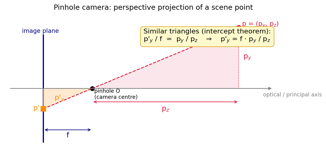
Pinhole projection: the scene point p, the pinhole O, the image plane at distance f, and the two shaded similar triangles that give p'_y = f·p_y/p_z. বাংলা: Pinhole projection-এর জ্যামিতি — scene point p, ছিদ্র O, দূরত্ব f-এ image plane, আর ছায়া দেওয়া দুটি সদৃশ ত্রিভুজ, যাদের অনুপাত থেকেই p'_y = f·p_y/p_z আসে।
The whole projection formula lives in this one picture. The big triangle (legs p_z and p_y) and the small triangle (legs f and p'_y) share the apex angle at O, so their sides are proportional. Note that the physical image is inverted (p' is below the axis when p is above); using the virtual image plane in front of O removes the flip.
বাংলা: পুরো formula এই এক ছবিতেই আছে — বড় আর ছোট ত্রিভুজের শীর্ষকোণ এক, তাই বাহু সমানুপাতিক। খেয়াল করুন আসল ছবি উল্টো হয় (p উপরে, p' নিচে); হিসাব সহজ করতে আমরা virtual image plane সামনে এনে ছবিটা সোজা করে নিই।
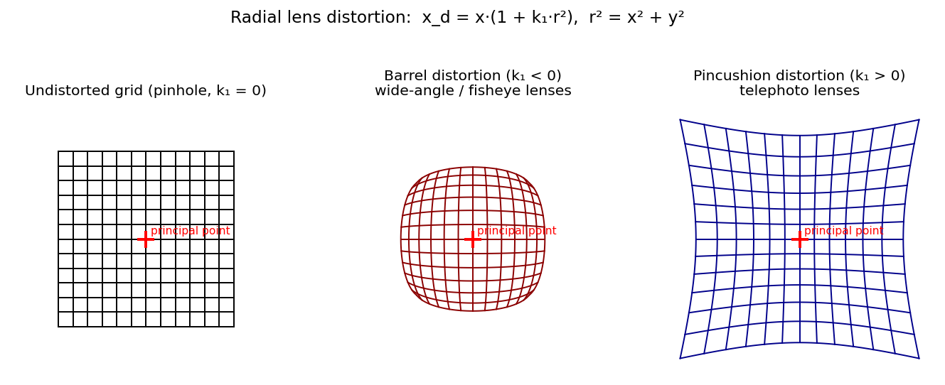
Radial distortion applied to a perfect grid: undistorted (k₁ = 0), barrel (k₁ < 0, wide-angle lenses), pincushion (k₁ > 0, telephoto lenses). The red cross is the principal point. বাংলা: একটা নিখুঁত grid-এ radial distortion: মাঝখানে barrel (k₁<0, লাইন বাইরে ফোলে — wide-angle lens), ডানে pincushion (k₁>0, লাইন ভেতরে বাঁকে — telephoto lens)। লাল চিহ্নটি principal point।
This is the exact figure to sketch in the exam ("Sketch a barrel distortion"). Distortion is zero at the principal point and grows with r² — compare how little the central lines bend versus the outer ones.
বাংলা: পরীক্ষায় "barrel distortion আঁকুন" এলে ঠিক এই ছবিটাই আঁকবেন: মাঝের লাইন প্রায় সোজা, বাইরের লাইন বেশি বাঁকা — কারণ distortion বাড়ে r²-এর সাথে।
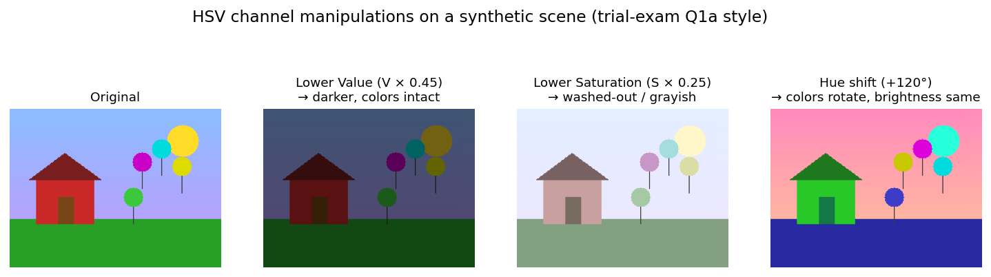
A synthetic scene and three HSV edits: lowering V darkens everything, lowering S washes colors toward gray, shifting H rotates all colors around the wheel while brightness stays put. This is trial-exam Q1a in picture form. বাংলা: একটি কৃত্রিম দৃশ্যে তিনটি HSV পরিবর্তন: V কমালে সব অন্ধকার হয়, S কমালে রঙ ধূসর হয়ে যায়, H ঘোরালে রঙগুলো রঙচক্রে ঘুরে যায় কিন্তু উজ্জ্বলতা অটুট থাকে — trial exam Q1a-র ছবি-রূপ।
Memorize the visual signatures: V-edit = same colors, darker; S-edit = same brightness, grayer; H-edit = different colors, same brightness. Given four thumbnails in the exam, classify by asking "did brightness change? did colorfulness change? did the colors themselves swap?"
বাংলা: তিনটে চিহ্ন মুখস্থ করুন: V কমা = একই রঙ কিন্তু অন্ধকার; S কমা = একই উজ্জ্বলতা কিন্তু ফ্যাকাশে; H ঘোরা = রঙ বদলে গেছে কিন্তু উজ্জ্বলতা একই। পরীক্ষায় ছবি মেলাতে এই তিন প্রশ্ন করুন নিজেকে।
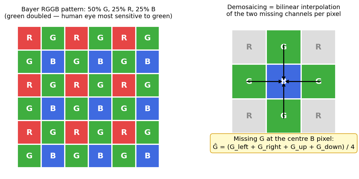
Left: the RGGB Bayer pattern — half the photosites are green. Right: demosaicing — the missing green at a blue pixel is the average of its four green neighbors. বাংলা: বাঁয়ে RGGB Bayer pattern — অর্ধেক pixel সবুজ। ডানে demosaicing — নীল pixel-এ অনুপস্থিত সবুজ মান তার চার প্রতিবেশী G-এর গড়।
One sensor, one value per site; color is a reconstruction. Whenever you see "raw image / aliasing artifacts / post-processing necessary" in a question, this picture is the answer.
বাংলা: Sensor আসলে রঙিন না — প্রতি ঘরে একটাই সংখ্যা; রঙ পরে গড় করে বানানো হয়। "Raw image-এ artifact কেন" জাতীয় প্রশ্নের উত্তর এই ছবি।
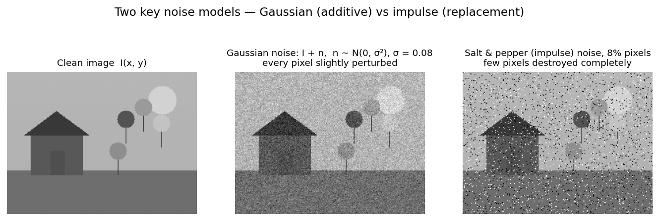
The same clean image corrupted two ways: Gaussian noise perturbs every pixel a little (σ = 0.08); impulse noise destroys a few pixels completely (8% set to pure black/white). বাংলা: একই ছবি দুইভাবে নষ্ট: Gaussian noise প্রতিটা pixel-কে একটু একটু নাড়ায়; salt & pepper অল্প কিছু pixel-কে পুরোপুরি সাদা/কালো করে দেয়।
The visual difference drives the filtering choice in Chapter 2: Gaussian noise → averaging/Gaussian filter; salt & pepper → median filter (an average would smear the extreme outliers into the neighborhood).
বাংলা: এই পার্থক্যই Chapter 2-এর filter পছন্দ ঠিক করে: Gaussian noise-এ গড়-জাতীয় filter, আর salt & pepper-এ median filter — কারণ গড় নিলে চরম মানগুলো আশেপাশে ছড়িয়ে যায়।
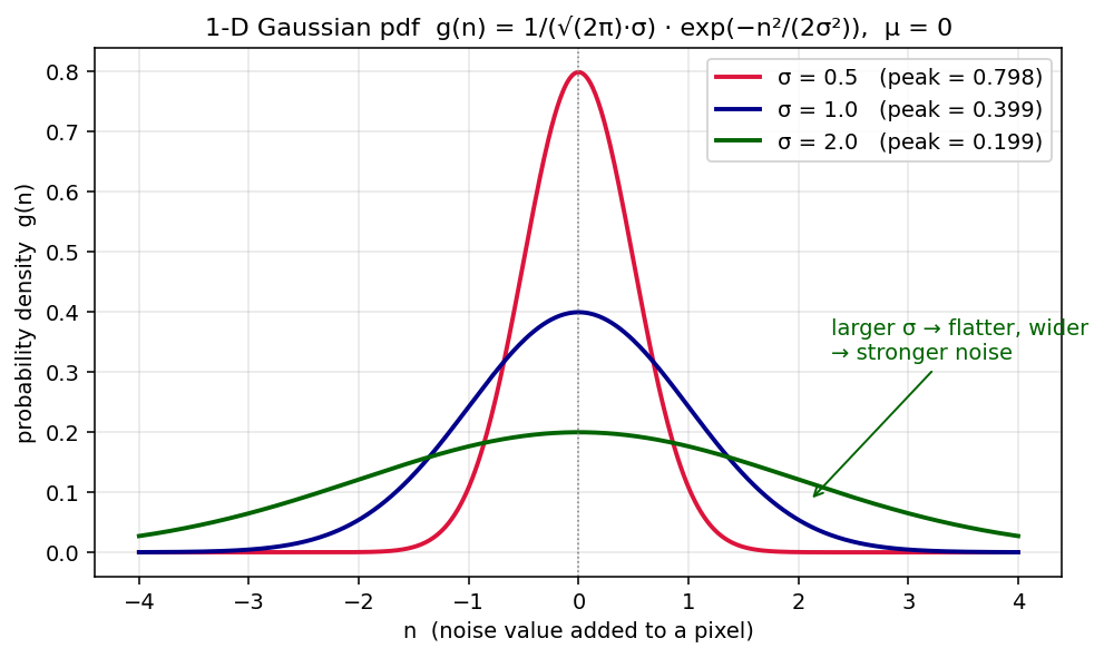
The Gaussian pdf for σ = 0.5, 1, 2 (μ = 0). Larger σ → wider and flatter bell — but the area under each curve is exactly 1. বাংলা: σ = 0.5, 1, 2-এর জন্য Gaussian pdf — σ বড় হলে ঘণ্টা চওড়া ও চ্যাপ্টা হয়, কিন্তু প্রতিটা curve-এর নিচের area ঠিক 1-ই থাকে।
Read the peak values: 0.798, 0.399, 0.199 — exactly \(1/(\sqrt{2\pi }\sigma )\). This figure doubles as the picture of the Gaussian filter kernel of Chapter 2.
বাংলা: Peak-এর মান 1/(√(2π)σ) সূত্র মেনে চলে — σ দ্বিগুণ, peak অর্ধেক। Chapter 2-এর Gaussian blur kernel-ও দেখতে ঠিক এই-ই।
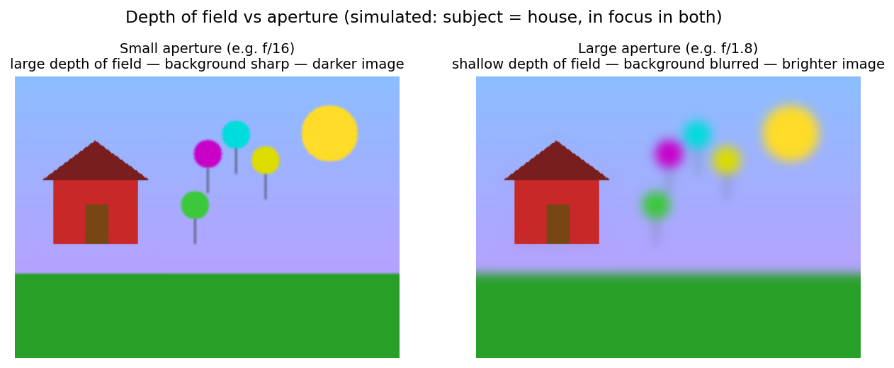
Simulated depth of field: small aperture (f/16) keeps house, balloons, and sun acceptably sharp; large aperture (f/1.8) isolates the house and melts the background — and would also yield a brighter image at the same exposure time. বাংলা: Depth of field-এর simulation: ছোট aperture-এ (f/16) সব মোটামুটি sharp; বড় aperture-এ (f/1.8) শুধু বাড়িটা sharp, background গলে গেছে — আর একই exposure time-এ ছবিটা উজ্জ্বলও হতো।
Connect to Section 4.8: large D → large blur circles for off-focal-plane objects → shallow DoF, plus 1/N² more light. The portrait/landscape trade-off in one image pair.
বাংলা: §4.8-এর সাথে মেলান: D বড় → focal plane-এর বাইরের বস্তুর blur-বৃত্ত বড় → DoF অগভীর, সাথে আলোও বেশি (1/N²)। Portrait বনাম landscape-এর পুরো trade-off এক জোড়া ছবিতে।
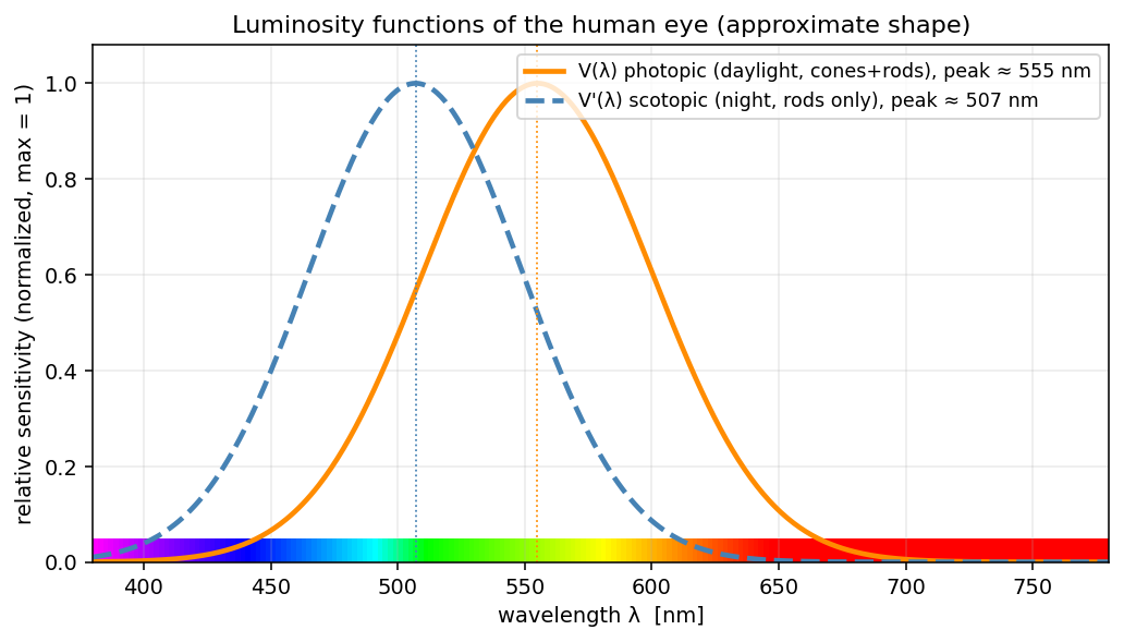
Approximate photopic V(λ) (daylight, peak ≈ 555 nm) and scotopic V′(λ) (night, peak ≈ 507 nm) sensitivity curves, with the visible spectrum strip below. বাংলা: আনুমানিক photopic V(λ) (দিন, peak ≈ 555 nm) আর scotopic V′(λ) (রাত, peak ≈ 507 nm) sensitivity curve, নিচে দৃশ্যমান বর্ণালির পটি।
At equal physical energy, yellow-green looks brightest and blue/deep red look dark — that is why Bayer doubles green and why luma formulas weight G highest. The night-time shift toward blue-green (Purkinje effect) follows from the V′ curve.
বাংলা: সমান শক্তিতে সবুজ-হলুদই সবচেয়ে উজ্জ্বল লাগে — সেজন্যই Bayer pattern-এ সবুজ দ্বিগুণ আর brightness-সূত্রে G-এর ওজন সবচেয়ে বেশি। রাতে peak নীল-সবুজের দিকে সরে — V′ curve-এর ফল।
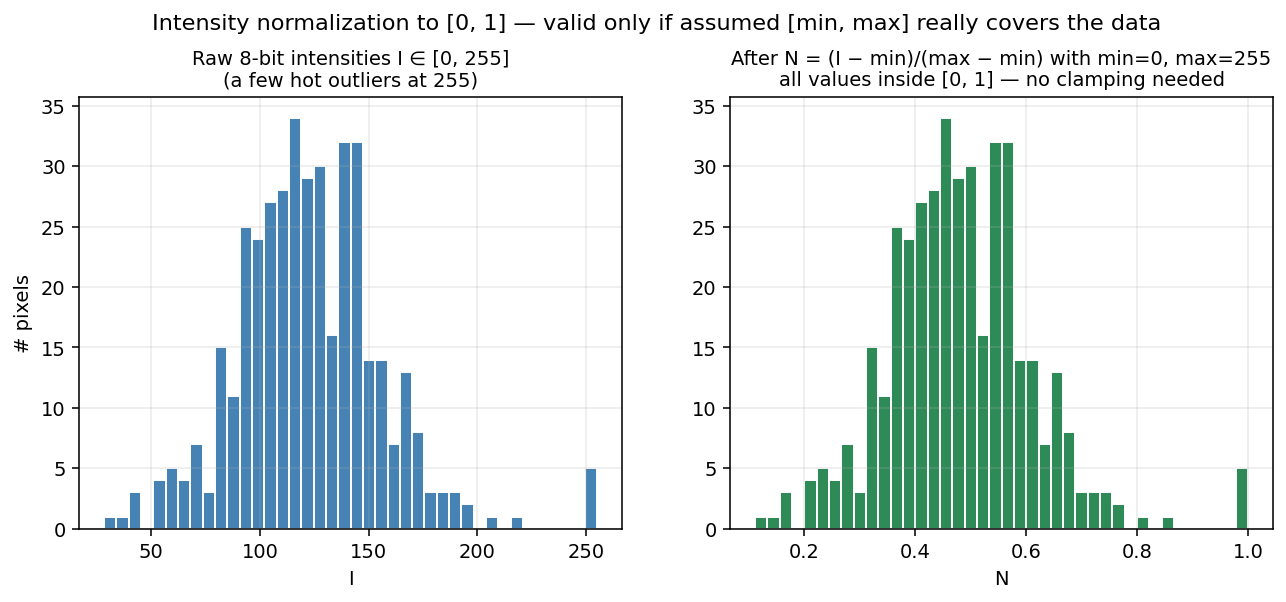
Left: raw 8-bit histogram with a few saturated outliers at 255. Right: after N = (I − min)/(max − min) with the assumed range [0, 255] — every value lands in [0, 1] because the assumed range really covers the data. বাংলা: বাঁয়ে কাঁচা 8-bit histogram (255-এ কিছু outlier)। ডানে normalization-এর পরে — ধরে নেওয়া range [0,255] data-কে সত্যিই cover করে বলে সব মান [0,1]-এ পড়েছে; নইলে clamp করতে হতো।
The shape of the histogram is preserved — normalization is affine. Only if the data exceeded the assumed range would clamping kick in and pile mass up at 1.0.
বাংলা: Histogram-এর আকৃতি একই থাকে — normalization affine বলেই। Data ধরে নেওয়া range ছাড়ালে তবেই clamp করতে হয়, আর তখন 1.0-তে একটা কৃত্রিম স্তূপ জমে।
§6 Algorithms & Code¶
6.1 Loading an image, BGR↔RGB, channel swap¶
"""
Purpose:
  Sheet 2 task 4 — load with OpenCV (BGR), convert to RGB,
  print stats, swap red/blue channels, save modified image.
Input:
  Color image file, e.g. img/hummingbird_from_pixabay.png
"""
import cv2
import numpy as np
import matplotlib.pyplot as plt

def show_image(img_bgr, title=""):
    img_rgb = cv2.cvtColor(img_bgr, cv2.COLOR_BGR2RGB)
    plt.imshow(img_rgb); plt.title(title); plt.axis("off"); plt.show()

def image_stats(img):
    h, w = img.shape[:2]
    c = 1 if img.ndim == 2 else img.shape[2]
    print(f"width={w}  height={h}  channels={c}  dtype={img.dtype}")

img = cv2.imread("hummingbird.png")
image_stats(img)
show_image(img, "original")

# swap red and blue channels = "blue bird"
blue_bird = img.copy()
blue_bird[..., [0, 2]] = blue_bird[..., [2, 0]]
cv2.imwrite("blue_hummingbird.png", blue_bird)
show_image(blue_bird, "blue_hummingbird")
Step-by-step. OpenCV reads in BGR order, so the index swap [0, 2] ↔ [2, 0] puts red where blue was and vice versa. We always convert to RGB before plotting because matplotlib expects RGB. image_stats enforces the lecture's rule: know your width/height/channels/dtype before computing.
Exam relevance. "Why does an image loaded with OpenCV look blue-ish in matplotlib?" → because OpenCV stores BGR while matplotlib interprets the array as RGB.
বাংলা: OpenCV ছবি পড়ে BGR ক্রমে, matplotlib আঁকে RGB ধরে — এই অমিলেই ছবি "নীলচে" দেখায়। তাই plot-এর আগে সবসময় cv2.cvtColor(img, cv2.COLOR_BGR2RGB)। আর channel swap মানে শুধু index অদলবদল — \([..., [0,2]] = [..., [2,0]]\)।
6.2 HSV hue shift¶
"""
Purpose: rotate hue without changing brightness/saturation.
Input: any BGR image, scalar offset in degrees.
"""
def hue_shift(img_bgr, hue_offset_deg):
    hsv = cv2.cvtColor(img_bgr, cv2.COLOR_BGR2HSV)
    # OpenCV stores H in [0, 180) for uint8 images → half-degrees!
    h = (hsv[..., 0].astype(np.int16) + hue_offset_deg // 2) % 180
    hsv[..., 0] = h.astype(np.uint8)
    return cv2.cvtColor(hsv, cv2.COLOR_HSV2BGR)

shifted = hue_shift(img, 120)   # rotate every color by 120°
Step-by-step. Convert to HSV, add the offset only to channel 0 (hue) with a modulo wrap at 180 (OpenCV packs 360° of hue into 0–179 so it fits a uint8), convert back. S and V are untouched, so perceived brightness stays constant — exactly the trial-exam Q1a "hue shift" case. The cast to int16 before adding prevents uint8 overflow.
বাংলা: Hue shift মানে শুধু channel 0-তে যোগ আর 180-তে modulo (OpenCV uint8-এ 360°-কে 0–179-এ ভাঁজ করে রাখে, তাই ডিগ্রিকে 2 দিয়ে ভাগ)। S, V অপরিবর্তিত — তাই উজ্জ্বলতা একই থেকে রঙ ঘুরে যায়। যোগের আগে int16-এ cast না করলে uint8 overflow-এ ফল ভুল হবে — এটা চিরাচরিত bug।
6.3 Pinhole projection (matches trial-exam Q4a)¶
def project_pinhole(P, f):
    """P = (x, y, z) in camera frame, f = focal length.
    Returns metric image-plane coordinates (x', y')."""
    x, y, z = P
    assert z != 0, "point at the pinhole plane cannot be projected"
    return (f * x / z, f * y / z)

def project_to_pixels(P, f, m_x, m_y, o_x, o_y):
    """Full pixel-coordinate projection u = m_x*f*x/z + o_x."""
    x, y, z = P
    return (m_x * f * x / z + o_x, m_y * f * y / z + o_y)

print(project_pinhole((10, 5, 3), 2))                    # (6.667, 3.333)
print(project_to_pixels((0.2, 0.1, 2.0), 0.005,
                        200_000, 200_000, 320, 240))     # (420.0, 290.0)
Failure case. \(z = 0\) → division by zero (point in the pinhole plane); \(z < 0\) → point behind the camera, formally projects but is invisible. Both are classic short-question traps.
বাংলা: দুটো function মনে রাখুন: project_pinhole দেয় মিটারে মাপা image-plane বিন্দু, আর project_to_pixels দেয় আসল pixel (m_x দিয়ে গুণ + principal point যোগ)। z = 0 হলে ভাগ অসম্ভব, z ঋণাত্মক হলে বিন্দু ক্যামেরার পেছনে — দুটোই পরীক্ষার ফাঁদ।
6.4 Adding Gaussian and salt-and-pepper noise¶
def add_gauss_noise(img_uint8, sigma=0.05, mu=0.0, rng=np.random.default_rng(0)):
    f = img_uint8.astype(np.float32) / 255.0          # work in [0,1] floats!
    noisy = f + rng.normal(mu, sigma, f.shape)        # I + n,  n ~ N(mu, sigma^2)
    return np.clip(noisy, 0.0, 1.0)                   # clamp back into range

def add_salt_pepper(img_uint8, p=0.05, rng=np.random.default_rng(0)):
    out = img_uint8.copy()
    m = rng.random(out.shape[:2])
    out[m < p / 2] = 0          # pepper
    out[m > 1 - p / 2] = 255    # salt
    return out
Step-by-step. Gaussian: convert to float (avoids uint8 wrap-around), add one normal sample per pixel, clip to [0, 1] — note the clip slightly biases very dark/bright regions, a subtle consequence of finite dynamic range. Salt & pepper: draw one uniform number per pixel; the lowest fraction p/2 becomes black, the highest p/2 becomes white — pixels are replaced, not perturbed.
বাংলা: Gaussian noise যোগ করার আগে অবশ্যই float-এ যান — uint8-এ 250 + 10 = 4 হয়ে যায় (wrap-around)! আর লক্ষ করুন: Gaussian noise মান যোগ করে, salt & pepper মান প্রতিস্থাপন করে — এই পার্থক্যটাই পরে median বনাম Gaussian filter বেছে নেওয়ার ভিত্তি।
6.5 Bilinear Bayer demosaicing (toy version)¶
def demosaic_green_at_blue(raw, x, y):
    """raw = single-channel Bayer mosaic; (x, y) = a blue photosite.
    Estimate the missing green as the mean of the 4-neighborhood."""
    return (int(raw[y, x-1]) + int(raw[y, x+1]) +
            int(raw[y-1, x]) + int(raw[y+1, x])) / 4
Note. Casting to int before summing prevents uint8 overflow (four values up to 255 sum to 1020 > 255). OpenCV's production version is cv2.cvtColor(raw, cv2.COLOR_BAYER_RG2BGR).
বাংলা: চার প্রতিবেশীর গড় — এটুকুই demosaicing-এর মূল ধারণা। যোগ করার আগে int-এ cast জরুরি, নইলে চারটা uint8-এর যোগফল overflow করবে।
6.6 Vignetting correction with a flat-field frame¶
def devignette(img, flat):
    """flat = photo of a uniformly white surface (flat-field frame)."""
    f = flat.astype(np.float32)
    scale = f.mean() / np.maximum(f, 1e-6)   # inverse per-pixel factor
    return np.clip(img.astype(np.float32) * scale, 0, 255).astype(np.uint8)
Theory link. The flat-field frame measures exactly how much each pixel is darkened by the lens; dividing by it (equivalently multiplying by its inverse, normalized by the mean) flattens the falloff — straight from the lecture's vignetting slide.
বাংলা: সাদা পৃষ্ঠের ছবিই বলে দেয় কোন pixel কতটা অন্ধকার হয়েছে; সেটার উল্টো অনুপাতে গুণ করলেই vignetting বাতিল। ভাগের আগে শূন্য এড়াতে np.maximum(f, 1e-6) — ছোট কিন্তু জরুরি সতর্কতা।
§7 Trial-Exam Mapping¶
| Trial-exam item | What you must know | Where in this chapter |
|---|---|---|
| Q1a HSV match | Decreasing V darkens; decreasing S grays out; hue shift rotates colors at constant brightness | §2.4, §4.6, HSV figure |
| Q1b printer/LED gap-fill | Printers ⇒ subtractive ⇒ CMYK; LEDs ⇒ additive ⇒ RGB | §2.4 |
| Q1c depth of field & aperture | Larger aperture ⇒ shallower DoF + brighter; smaller aperture ⇒ larger DoF + darker (secondary effect: brightness/exposure) | §2.9, §4.8, DoF figure |
| Q1d barrel distortion sketch | Wide-angle/fisheye; straight lines bow outward; distortion grows with r² from the principal point | §2.11, §4.5, distortion figure |
| Q4a perspective projection | \(p' = f\cdot p/p_{z}\); with p = (10, 5, 3), f = 2 → (20/3, 10/3) | §4.1, §6.3 |
Model gap-fill sentence (Q1b): "When thinking about printers, we need to use subtractive color spaces, such as CMYK. This is in contrast to what happens with LEDs, where we need to think about additive color spaces, such as RGB."
Model short answer (Q1c): "Increasing the aperture (smaller f-number) reduces the depth of field — fewer parts of the scene are in focus — and lets more light reach the sensor, so the image becomes brighter. Decreasing the aperture does the opposite: larger depth of field but a darker image."
The fully graded answers are in CVML_Trial_Exam_Analysis.md.
§8 Mock Exam — 20 Questions¶
Answer everything on paper first; full worked solutions follow in §8.5. Tier A = basics, B = intuition, C = harder computation/derivation, D = transfer questions slightly beyond the lecture (typical for a tough oral or a "Transfer" section in the written exam).
Tier A — Basic (definitions & direct formula use)¶
A1. Define digital image, pixel, and channel. State the number of channels in: a grayscale image, an RGB image, an RGBA image, a CMYK image.
A2. An image is converted to HSV and edited. Match each edit to its visual effect: (i) V multiplied by 0.4, (ii) S multiplied by 0.2, (iii) H shifted by 120°. Effects: (a) colors become washed-out/grayish, (b) all colors change but brightness stays, © the image becomes darker.
A3. Project the point \(p = (6, 9, 3)\) with a pinhole camera of focal length \(f = 2\). Give \(p' = (p'_{x}, p'_{y})\).
A4. Normalize the intensity \(I = 64\) from the range [0, 255] (a) to [0, 1] and (b) to \([-1, 1]\). Give 3 decimal places.
A5. Fill the gaps: "Printers use ______ color spaces such as ______, because adding pigments makes the result ______. Displays use ______ color spaces such as ______, because adding light makes the result ______."
Tier B — Intuitive (why / when)¶
B6. Why does the Bayer pattern contain twice as many green filters as red or blue? And why is post-processing unavoidable with a Bayer sensor?
B7. A photographer stops down from f/2 to f/16 and the photo becomes sharp from front to back, but also dark. Explain both effects from the geometry of the aperture, and name the two compensation options together with the new problem each one introduces.
B8. Why do computer-vision algorithms prefer floating-point intensities in [0, 1] over uint8 values in [0, 255]? Name at least three reasons mentioned in the lecture.
B9. Real cameras have lenses, not pinholes. Why do we nevertheless base the whole course on the pinhole model, and what do we do to real images so that the model applies?
B10. Explain the physical origin of (a) streaking/blooming in CCD chips and (b) the rolling-shutter effect in CMOS chips. For each, give one situation where the artifact ruins the photo.
Tier C — Harder (multi-step computation / derivation)¶
C11. Derive \(p'_{y} = f\cdot p_{y}/p_{z}\) from similar triangles (sketch + every algebraic step). Then compute the pixel coordinates of \(p = (0.3, -0.2, 1.5)\) m for a camera with \(f = 6 mm\), square pixels of size 10 µm, and principal point (320, 240).
C12. A lens has radial distortion \(k_{1} = -0.25\) (and \(k_{2} = 0\)). For the undistorted points \(A = (0.5, 0)\) and \(B = (1.0, 0)\) (normalized, principal point at origin), compute the distorted positions. Which distortion type is this? Show numerically that the spacing between A and B is compressed non-uniformly, and explain why straight lines therefore curve.
C13. Gaussian noise with μ = 0 and σ = 2 gray levels is added to every pixel of an 8-bit image. (a) Evaluate the noise pdf at n = 0. (b) What fraction of pixels is corrupted by more than 4 gray levels? © On a 1-megapixel image, roughly how many pixels deviate by more than 6 gray levels? (Use the 68–95–99.7 rule.)
C14. A 30 m tall tower stands 600 m from a camera with a 50 mm lens. (a) How tall is the tower's image on the sensor (in mm)? (b) How many pixels is that with 5 µm pixels? © At what distance would the tower exactly fill a 24 mm tall sensor?
C15. Convert \(RGB = (0.2, 0.8, 0.4)\) to HSV by hand (show V, Δ, S, H). Then prove with a concrete counterexample that the RGB→HSV map is not linear.
Tier D — Transfer (adjacent to, but beyond, the lecture)¶
D16. The lecture models noise with an isotropic Gaussian. Write down the pdf of a general 2-D Gaussian with covariance matrix Σ, and explain the difference between the isotropic case \(\Sigma = \sigma ^{2}\cdot I\) and an anisotropic diagonal case \(\Sigma = \operatorname{diag}(\sigma _{1}^{2}, \sigma _{2}^{2})\). Give one physically plausible camera scenario where the noise (or blur) would be anisotropic.
D17. The pinhole has no focus; real lenses obey the thin-lens equation \(1/f = 1/z + 1/z'\) (object distance z, image distance z′, both measured from the lens). (a) For \(f = 50 mm\) and an object at \(z = 200 mm\), where must the sensor sit? (b) Show that for \(z \to \infty\) the thin lens behaves exactly like a pinhole camera with image plane at distance f. © What happens to the image as \(z \to f\) from above?
D18. The lecture only covers perspective projection. Define orthographic projection and the weak-perspective approximation. An object spans depths \(z \in [99, 101]\) (camera units, f = 0.05). Compute the perspective scale \(f/z\) at both depth extremes, compare with the weak-perspective scale \(f/\bar{z}\) at the mean depth, and give the maximum relative error. When is weak perspective a good model?
D19. Photon arrival is actually a counting process: the number of photons k collected by a pixel follows a Poisson distribution with mean N (variance also N). (a) Show that the signal-to-noise ratio is \(SNR = \sqrt{N}\). (b) Compute the SNR for N = 100 and N = 10,000 photons. © Explain why this "shot noise" looks approximately Gaussian for large N, and why dark image regions are noisier than bright ones — connecting to the lecture's "underexposure ⇒ bad SNR" statement.
D20. Cameras usually store gamma-encoded values I_enc = I_lin^(1/2.2) instead of linear intensities. (a) Is this transformation linear? (b) Two scene patches have linear intensities 0.2 and 0.8. Compute the gamma-encoded value of their true average, and the average of their gamma-encoded values (3 decimals each). © What does the mismatch imply for naively averaging (e.g. blurring) gamma-encoded images?
§8.5 Solutions¶
Tier A¶
A1.
A digital image is a 2-D array of scalar values (equivalently a function I(x, y) returning the stored value(s) at each position). A pixel (picture element) is one cell of that array. A channel is one value-layer per pixel — with c channels each pixel stores a c-vector.
Channel counts: grayscale = 1, RGB = 3, RGBA = 4, CMYK = 4.
বাংলা: ছবি = সংখ্যার 2-D grid, pixel = তার একটা ঘর, channel = প্রতি ঘরে রাখা মানের স্তর — gray ১টা, RGB ৩টা, RGBA আর CMYK ৪টা করে।
A2. (i) → ©: V is brightness; scaling it down darkens everything while hue and saturation stay. (ii) → (a): S is purity; reducing it mixes colors toward gray (washed-out look) at unchanged brightness. (iii) → (b): H is the color-wheel angle; shifting rotates every color (red→green→blue) while V — the perceived brightness — is untouched. বাংলা: V কমা = অন্ধকার, S কমা = ফ্যাকাশে/ধূসর, H ঘোরা = রঙ বদল কিন্তু উজ্জ্বলতা অটুট — এই তিন লাইনই উত্তর।
A3.
বাংলা: Formula-তে বসিয়ে depth দিয়ে ভাগ — p' = (4, 6)। ভাগটা p_z দিয়ে, f দিয়ে নয় — এটাই সাধারণ ভুল।
A4.
বাংলা: [0,1]-এ গেলে শুধু 255 দিয়ে ভাগ; [−1,1]-এ গেলে আগে [0,1], তারপর ×2 −1। 64 মাঝামাঝির নিচে, তাই উত্তর ঋণাত্মক হওয়াটাই যুক্তিসঙ্গত।
A5. "Printers use subtractive color spaces such as CMYK, because adding pigments makes the result darker. Displays use additive color spaces such as RGB, because adding light makes the result brighter." বাংলা: Pigment যোগ = আলো শোষণ বাড়ে = কালচে (subtractive, CMYK); আলো যোগ = উজ্জ্বল (additive, RGB)। Printer-CMYK, LED-RGB — জোড়াটা মুখস্থ।
Tier B¶
B6. Green is doubled because the human eye is most sensitive to green — the photopic luminosity curve V(λ) peaks near 555 nm, and most of our perceived luminance/detail comes from the green band. Doubling green sampling makes the channel that matters most for sharpness the best-sampled one. Post-processing is unavoidable because each photosite measures only one of R, G, B; the other two channels at every pixel do not exist in the raw data and must be interpolated from neighbors (demosaicing). Additional consequences: unequal color information, aliasing/color artifacts at fine structures. বাংলা: চোখ সবুজে সবচেয়ে সংবেদনশীল বলে সবুজ filter দ্বিগুণ; আর প্রতি pixel-এ মাত্র এক রঙ মাপা হয় বলে বাকি দুই রঙ interpolate করতেই হয় — raw data-তে সেগুলো নেই-ই।
B7. Sharpness: the blur disc of an off-focal-plane point is a slice of the light cone leaving the lens; its diameter is proportional to the aperture diameter D (\(c = D\cdot |z'_{s} - z'_{p}|/z'_{p}\)). Stopping down from f/2 to f/16 shrinks D by 8×, hence every circle of confusion by 8× — points far from the focal plane now fall below the "looks sharp" threshold → depth of field extends front to back. Darkness: the light gathered is proportional to the aperture area, \(E \propto D^{2} \propto 1/N^{2}\); from f/2 to f/16 the image receives \((16/2)^{2} = 64\times\) less light → dark image. Compensations: (1) longer exposure time → risk of motion blur (camera shake, moving subjects); (2) higher ISO/gain → amplifies sensor noise → grainy image (bad SNR). বাংলা: ছোট aperture → blur-বৃত্ত ছোট → সব sharp, কিন্তু আলো ঢোকে D²-অনুপাতে কম → অন্ধকার। ক্ষতিপূরণের দুই পথ, দুটোরই দাম: exposure বাড়ালে motion blur, ISO বাড়ালে noise।
B8. (1) Higher precision — float granularity is far finer than 256 levels, so chained operations don't accumulate rounding error as fast. (2) No overflow/underflow bugs — uint8 arithmetic wraps (250 + 10 = 4), floats don't; fewer programming errors. (3) Uniform convention across algorithms — thresholds, weights, probabilities all live naturally in [0, 1]; intermediate results of convolutions or ML normalizations stay representable. Cost (also lecture-mentioned): higher memory consumption. বাংলা: Float [0,1]-এর তিন সুবিধা: precision বেশি, overflow/underflow নেই, আর সব algorithm-এর সাথে এক convention। দাম একটাই — memory বেশি লাগে।
B9. The pinhole model gives clean, linear (ray-optics) geometry: scene point, pinhole, and image point are collinear, projection is a one-line formula, straight world lines stay straight. All later machinery (calibration matrices, epipolar geometry, triangulation, homographies) is built on this linearity. Real lenses add radial distortion, vignetting, blur, etc., so we calibrate the camera (estimate f, principal point, k₁, k₂, …) and undistort/rectify the images — computationally bending the recorded image back to what an ideal pinhole would have seen. After that, pinhole math applies to real photos. বাংলা: Pinhole-এর অঙ্ক সরল ও linear বলে পুরো course ওটার উপর দাঁড়িয়ে; বাস্তব lens-এর দোষগুলো আমরা calibration দিয়ে মেপে undistort করে ছবিকেই pinhole-সদৃশ বানিয়ে নিই — model-কে জটিল করার বদলে data-কে শোধরাই।
B10. (a) CCD streaking/blooming: a CCD reads out by physically shifting charge row-by-row across the chip. During shifting, photons keep arriving, so a very bright source keeps injecting charge into the pixels passing under it → bright vertical streaks; and when a photosite's charge well overflows, surplus charge spills into neighbors → blooming. Ruins e.g. night shots with car headlights or the sun in frame. (b) CMOS rolling shutter: rows are exposed and read at different times — the shutter "falls" down the frame. Fast-moving objects move between row exposures, so shapes shear/bend (helicopter blades become curved, "Jello effect" in videos). Serious problem in sports photography (lecture's example) and on vibrating platforms (drones). বাংলা: CCD-তে charge সরানোর সময়েও আলো পড়তে থাকে বলে উজ্জ্বল উৎসে লম্বা streak/blooming; CMOS-এ প্রতিটা সারি ভিন্ন সময়ে exposed হয় বলে দ্রুতগতির জিনিস বেঁকে যায় (rolling shutter)। Streak ↔ CCD, বাঁকা পাখা ↔ CMOS — জোড়া মেলান।
Tier C¶
C11. Derivation. Place the pinhole at the origin O, optical axis = z. Image plane at distance f. The ray from scene point p = (·, p_y, p_z) through O hits the image plane at height p'_y. The triangle (O, axis-foot at depth p_z, point at height p_y) and the triangle (O, axis-foot at depth f, image point at height p'_y) are both right triangles sharing the angle at O ⇒ similar ⇒ corresponding sides proportional:
Numbers. \(f = 6 mm = 0.006 m\); pixel size 10 µm ⇒ \(m = 1/10^{-5} = 100,000 px/m\) ⇒ \(f_{x} = f_{y} = m\cdot f = 0.006 \cdot 100,000 = 600 px\).
u = f_x · p_x/p_z + o_x = 600 · (0.3 / 1.5) + 320 = 600 · 0.2  + 320 = 120 + 320 = 440
v = f_y · p_y/p_z + o_y = 600 · (−0.2 / 1.5) + 240 = 600 · (−0.13̄) + 240 = −80 + 240 = 160
pixel = (440, 160)
(Negative metric y maps above the principal point in this convention — consistent, since v = 160 < 240.) বাংলা: আগে সদৃশ ত্রিভুজ থেকে p'_y = f·p_y/p_z, তারপর pixel-এ যেতে m দিয়ে গুণ আর principal point যোগ — দুই ধাপের কোনোটাই বাদ দিলে পুরো নম্বর নেই। উত্তর (440, 160)।
C12.
A = (0.5, 0):  r² = 0.25  →  factor = 1 + (−0.25)(0.25) = 1 − 0.0625 = 0.9375
               A_dist = (0.5 · 0.9375, 0) = (0.46875, 0)
B = (1.0, 0):  r² = 1.0   →  factor = 1 + (−0.25)(1.0)  = 0.75
               B_dist = (0.75, 0)
\(k_{1} < 0\) and all points move toward the principal point ⇒ barrel distortion (wide-angle behavior). Spacing: undistorted gap B − A = 0.5; distorted gap = 0.75 − 0.46875 = 0.28125 — compressed to 56% — while near the center a gap of 0.5 (from 0 to A) only shrinks from 0.5 to 0.46875 (94%). The compression grows with radius. A straight world line sampled at many points gets each point pulled inward by a different amount (∝ r²), so the image of the line cannot remain straight — its outer parts sag toward the center more than its middle, producing the outward-bowed barrel look of grid lines. বাংলা: কেন্দ্রের কাছে সংকোচন মাত্র ৬%, বাইরে ৪৪% — এই অসমতাই রহস্য। সব বিন্দু সমান টানা হলে লাইন সোজাই থাকত; r²-অনুপাতে টানা হয় বলেই লাইন বেঁকে barrel হয়।
C13. (a)
(b) "More than 4 gray levels" = beyond 2σ. \(P(|n| > 2\sigma ) = 1 - 0.9545 = 0.0455\) → ≈ 4.6% of all pixels. © "More than 6 gray levels" = beyond 3σ. \(P(|n| > 3\sigma ) = 1 - 0.9973 = 0.0027\); on 10⁶ pixels: \(0.0027 \cdot 10^{6} = 2700\) → ≈ 2700 pixels. বাংলা: σ-এর গুণিতকে ভাবলেই সমাধান এক লাইনের: 2σ-র বাইরে ~4.6%, 3σ-র বাইরে ~0.27% — megapixel ছবিতে সেটাই ~২৭০০ pixel। 68–95–99.7 মুখস্থ থাকলে এ ধরনের প্রশ্ন free points।
C14. (a)
(b)
© Solve \(0.05 \cdot 30 / z = 0.024\):
বাংলা: একই সূত্র তিনবার, শুধু কোন রাশিটা অজানা সেটা বদলায়: ছবির উচ্চতা 2.5 mm, pixel-এ 500, আর sensor ভরাতে টাওয়ারকে আসতে হবে 62.5 m-এ। একক-রূপান্তরে (m ↔ mm ↔ µm) ভুলই এখানে একমাত্র বিপদ।
C15.
V = max(0.2, 0.8, 0.4) = 0.8
Δ = 0.8 − 0.2 = 0.6
S = Δ/V = 0.6/0.8 = 0.75
max = G ⇒ H = 60°·(2 + (B − R)/Δ) = 60°·(2 + (0.4 − 0.2)/0.6) = 60°·(2 + 1/3) = 140°
HSV = (140°, 0.75, 0.8)
Non-linearity: linearity would require \(V(a + b) = V(a) + V(b)\). Take \(a = (1,0,0)\), \(b = (0,1,0)\): \(V(a) + V(b) = 1 + 1 = 2\), but \(V(a+b) = \max (1,1,0) = 1 \neq 2\). Since already the V component violates additivity (max is not additive, and H is even piecewise-defined by which channel is largest), the map cannot be linear. ∎ বাংলা: ধাপে ধাপে: V হলো max, S হলো ফারাক-ভাগ-max, H ঠিক হয় কোন channel বড় তার সূত্রে — এখানে G বড় তাই 2-এর ঘর। আর non-linearity দেখাতে এক লাইনের counterexample: লাল+সবুজ=হলুদ, কিন্তু max যোগ মানে না (1+1≠1)।
Tier D¶
D16. General 2-D Gaussian pdf with mean μ ∈ ℝ² and covariance Σ (2×2, symmetric positive definite):
Isotropic \(\Sigma = \sigma ^{2}\cdot I\): det Σ = σ⁴, Σ⁻¹ = I/σ², so the exponent reduces to \(-(x^{2}+y^{2})/(2\sigma ^{2})\) — the formula from §4.4; level sets are circles, the noise/blur is direction-independent. Anisotropic diagonal \(\Sigma = \operatorname{diag}(\sigma _{1}^{2}, \sigma _{2}^{2})\): pdf factor \(1/(2\pi \sigma _{1} \sigma _{2}) \cdot \exp (-x^{2}/(2\sigma _{1}^{2}) - y^{2}/(2\sigma _{2}^{2}))\); level sets are axis-aligned ellipses — different strength along x and y. (A non-diagonal Σ rotates the ellipse.) Camera scenario: row-wise sensor readout can leave different noise statistics along rows vs. columns (fixed-pattern/readout noise is row-correlated); equally good answer: motion blur smears the point-spread function along the motion direction only, which is modeled as an anisotropic (elongated) Gaussian. বাংলা: Isotropic মানে সব দিকে সমান σ — contour বৃত্ত; anisotropic মানে দিকভেদে আলাদা σ — contour উপবৃত্ত। বাস্তব উদাহরণ: sensor-এর সারি-ভিত্তিক readout noise বা একদিকে টানা motion blur — দুটোই দিক-নির্ভর, তাই anisotropic model লাগে।
D17. (a)
(b) As \(z \to \infty\), the term \(1/z \to 0\), so \(1/z' \to 1/f\), i.e. \(z' \to f\): all sufficiently distant objects focus on a plane at distance f — exactly the pinhole geometry with image plane at f. The pinhole model is the far-field limit of the thin lens. © As \(z \to f^{+}\), \(1/z' = 1/f - 1/z \to 0^{+}\), so \(z' \to \infty\): the image plane needed for focus recedes to infinity (rays leave the lens parallel). Objects at or inside the focal length cannot be focused on any real sensor plane (a virtual image forms — the magnifying-glass regime). বাংলা: Thin-lens সূত্রে 1/f = 1/z + 1/z′ — বসিয়ে z′ = 200/3 ≈ 66.67 mm। z অসীমে গেলে z′ → f, অর্থাৎ দূরের জগতের জন্য lens-ক্যামেরা pinhole-এরই সমান — এজন্যই pinhole model এত ভালো কাজ করে। আর z → f হলে z′ → ∞ — focus আর সম্ভবই না।
D18.
Orthographic projection drops depth entirely: \(x' = p_{x}, y' = p_{y}\) (parallel rays, no division by z — formally the limit of moving the camera infinitely far away while zooming in). Weak perspective is the practical version: divide by one common mean depth z̄ instead of each point's own z: \(x' \approx (f/\bar{z})\cdot p_{x}\) — a single global scale.
Numbers (f = 0.05):
scale at z =  99:  f/z = 0.05/99  ≈ 0.00050505
scale at z = 101:  f/z = 0.05/101 ≈ 0.00049505
weak-perspective:  f/z̄ = 0.05/100 = 0.00050000
max relative error ≈ |0.00050505 − 0.00050000| / 0.00050505 ≈ 0.0100 ≈ 1%
When good: when the depth variation within the object is small compared to its distance (Δz ≪ z̄) — e.g. telephoto shots, far-away objects, face at 5 m. Then perspective foreshortening across the object is negligible and the projection is just a uniform scaling, which makes many recognition/geometry algorithms linear. বাংলা: Orthographic মানে z-কে পুরো অগ্রাহ্য; weak perspective মানে সবার জন্য একটাই গড় depth দিয়ে ভাগ। বস্তুর গভীরতার তারতম্য তার দূরত্বের তুলনায় ছোট হলে (এখানে ±1% ভুল) এই সরলীকরণ চমৎকার চলে — telephoto বা দূরের দৃশ্যে।
D19. (a) For Poisson, mean = N and variance = N, so the noise standard deviation is √N. Define SNR = signal/noise-std:
(b)
(100× more photons ⇒ only 10× better SNR — SNR grows with the square root of light.) © By the central limit theorem, a Poisson(N) variable is approximately Normal(N, N) for large N — sums of many independent photon arrivals smooth into a bell curve; that is why the lecture's additive-Gaussian model works well in decently lit images. In dark regions N is small: the relative fluctuation \(\sqrt{N}/N = 1/\sqrt{N}\) is large, so dark/underexposed areas look grainy — precisely the lecture's "too few photons → noise when scaled → bad signal-to-noise ratio." বাংলা: Photon গোনা Poisson process — গড় N হলে ছড়ানোও √N, তাই SNR = √N। আলো ১০০ গুণ বাড়ালে SNR মোটে ১০ গুণ বাড়ে। N বড় হলে Poisson ≈ Gaussian (central limit theorem) — তাই lecture-এর Gaussian model বৈধ; আর N ছোট (অন্ধকার অংশ) হলে আপেক্ষিক ওঠানামা 1/√N বড় — অন্ধকার ছবিই বেশি noisy।
D20. (a) No — \(I^(1/2.2)\) is a power law, and \((a + b)^\gamma \neq a^\gamma + b^\gamma\) in general; it is a pointwise non-linear mapping. (b)
True linear average:        (0.2 + 0.8)/2 = 0.5
Gamma-encode the average:    0.5^(1/2.2)  = 0.5^0.4545 ≈ 0.730

Encode first:                0.2^0.4545 ≈ 0.481      0.8^0.4545 ≈ 0.904
Average of encoded values:  (0.481 + 0.904)/2 ≈ 0.692

0.692 ≠ 0.730  — the two orders of operation disagree.
© Any algorithm that averages pixel values (Gaussian blur, downscaling, alpha blending, demosaicing) silently assumes linear intensities. Run it on gamma-encoded values and the result is systematically too dark around bright–dark transitions (0.692 < 0.730 here) — edge halos and wrong colors in blends. Correct pipeline: decode to linear (\(I^2.2\)), process, re-encode. This is the deeper meaning of the lecture's warning to know the meaning of your channel values, not just their range. বাংলা: Gamma encoding একটা power law — non-linear, তাই "আগে গড় পরে encode" আর "আগে encode পরে গড়" এক না (0.730 বনাম 0.692)। Blur/resize-এর মতো গড়-নির্ভর কাজ gamma-encoded ছবিতে সরাসরি চালালে ফল একটু বেশি অন্ধকার হয় — আগে linear-এ ফিরুন, কাজ সেরে আবার encode করুন।
§9 Exam-Day Cheat Sheet¶
Definitions in one breath
- Digital image = 2-D array of scalar values; pixel = one cell; channels = values per pixel (gray 1, RGB 3, RGBA/CMYK/RGBD 4).
- Origins: image formats & OpenCV — top-left, y down; graphics textures — bottom-left, [0,1]²; vision/3-D — principal point, [−1,1]². NumPy indexes
img[y, x]. - Dynamic range = span of representable values; editing tools [0, 255] (1 byte), CV algorithms float [0, 1] (precision, no over/underflow). Know range + meaning + dtype of every channel.
Color
- RGB additive (LED/display) · CMYK subtractive (printer/pigment) · HSV artistic (H angle, S purity, V brightness) · Lab/Luv perceptual (Euclidean distance ≈ perceived difference, decorrelated channels).
- HSV edits: V↓ darker · S↓ grayer · H-shift rotates colors at constant brightness.
- Color = reflected light; perception = ∫ L(λ)·R(λ)·V(λ) dλ ⇒ metamerism possible.
- Eye: rods (intensity, night) + 3 cone types L/M/S (⇒ 3-channel displays suffice). V(λ) peaks ≈ 555 nm (photopic), V′(λ) ≈ 507 nm (scotopic).
Geometry
p'_x = f·p_x/p_z     p'_y = f·p_y/p_z          (similar triangles; divides by depth!)
u = m_x·f·p_x/p_z + o_x                         (pixels = metric × density + principal point)
x_dist = x·(1 + k₁r² + k₂r⁴),  r² = x² + y²     (k₁<0 barrel/wide-angle, k₁>0 pincushion/tele)
N = f/D    E ∝ 1/N²    c ∝ D                    (f-number, light, circle of confusion)
- Large aperture (small N): bright + shallow DoF. Small aperture (large N): dark + deep DoF. Compensations: longer exposure → motion blur; higher ISO → noise.
- Pinhole assumptions vs reality: central projection ↔ aberrations/vignetting; ray optics ↔ finite aperture/circle of confusion; infinite DoF ↔ blur; instant exposure ↔ motion blur/rolling shutter; infinite dynamic range ↔ blooming/clipping; linear exact response ↔ noise/quantization.
Sensors & noise
- Bayer RGGB: 50% green (eye most sensitive there); demosaic by averaging same-color neighbors; artifacts at fine textures.
- CCD: linear, blooming + streaks (readout while exposed). CMOS: cheap, low-power, rolling shutter (rows exposed at different times).
- Normalization \(N = (I - \min )/(\max - \min )\); guaranteed in range only if [min, max] covers the data — otherwise clamp (lossy!).
- Gaussian noise: \(I_{noisy} = I + n, n ~ N(\mu , \sigma ^{2})\); pdf \(1/(\sqrt{2\pi }\sigma )\cdot \exp (-(n-\mu )^{2}/(2\sigma ^{2}))\); 68–95–99.7 at 1σ/2σ/3σ. Impulse noise: isolated pure black/white pixels (broken photosites).
- Quantization: spatial (pixel width Δx) + intensity (2⁸ = 256 levels) — unrecoverable, prevent at acquisition.
Quick traps
- OpenCV is BGR, matplotlib is RGB. OpenCV uint8 hue runs 0–179.
- DoF goes UP when aperture goes DOWN (N up). Big f-number = small hole.
- Projection divides by p_z (not by f). Pixels need m_x and o_x on top.
- uint8 wraps: 250 + 10 = 4. Cast to float/int16 before arithmetic.
- max() is not linear ⇒ RGB→HSV is not a matrix.
বাংলা মন্ত্র (শেষ মুহূর্তের জপ)
- "Projection মানে depth দিয়ে ভাগ: p' = f·p/p_z — দূরের জিনিস ছোট, depth হারিয়ে যায়।"
- "Aperture বড় → আলো বেশি, DoF কম; aperture ছোট → আলো কম, DoF বেশি — আর secondary effect-টা বলতে ভুলো না।"
- "Barrel মানে বাইরে ফোলা, wide-angle; pincushion মানে ভেতরে বাঁকা, telephoto; দোষ বাড়ে r²-এর সাথে।"
- "CMYK ছাপে (subtractive), RGB জ্বলে (additive); V কমলে অন্ধকার, S কমলে ফ্যাকাশে, H ঘুরলে রঙবদল।"
- "Gaussian noise যোগ হয়, salt & pepper বসে যায় — প্রথমটায় গড়-filter, দ্বিতীয়টায় median।"
- "Normalize আগে, কিন্তু range না মিললে clamp — আর clamp মানেই তথ্যের মৃত্যু।"
Final mantra: "f·p over p_z. Big aperture, small DoF, bright image. Barrel = wide-angle = bulge outward. CMYK prints, RGB lights up. Green is king on the Bayer grid."