Chapter 09 — Video Matching, Morphing & View Synthesis¶
Exam weight: ~10 / 110 points in the trial exam (Q8a: explain the view-morphing formula, Q8b: how rectification helps stereo processing, Q8c: three True/False on video matching, cross-dissolve, and physically valid morphs). Beginner-friendly, math-deep notes for the SS 2025 CVML exam at TU Braunschweig.
§1 Chapter Roadmap¶
This chapter answers one deceptively simple question: how do you smoothly transition from one image (or video) to another? The cheapest answer is the cross-dissolve \(M(t) = (1-t)\cdot I_{1} + t\cdot I_{2}\) — a pure color blend with zero geometric alignment, which produces ugly ghosting (double edges) the moment the two images are not pixel-aligned. The professional answer is morphing: first warp both images toward a shared intermediate geometry using a dense correspondence field, then cross-dissolve — the lecture formula is \(I_{M}(t) = (1-t)\cdot (t\cdot F_{1}\to _{2} \circ I_{1}) + t\cdot ((1-t)\cdot F_{2}\to _{1} \circ I_{2})\). To get correspondences between two videos shot with shaky handheld cameras, Sand & Teller's video matching finds, for every frame of video 1, the most similar frame of video 2 (dissimilarity \(D = \lambda \cdot p^{2} + m^{2}\) from parallax change and motion magnitude) and warps it into alignment — enabling effects like object removal, HDR video, and the TU Braunschweig Virtual Video Camera (a tetrahedralized space-time cube of frames, navigated by morphing). The punchline of the chapter is a warning: all of this is visually plausible but physically inconsistent — linear interpolation of pixel positions does not correspond to any real camera. Seitz & Dyer's view morphing fixes it: rectify the two views onto a common image plane (homographies H₁, H₂), interpolate linearly there (which exactly equals a real camera sliding along the baseline), and map back: \(\hat{x} = H_{1}^{-1}(H_{1}x + t\cdot (H_{2}x' - H_{1}x))\) — the trial-exam Q8a formula. The chapter leans heavily on earlier material: optical flow / brightness constancy (Chapter 6) supplies the dense correspondences, backward warping + bilinear sampling (Chapter 7) supplies the resampling machinery, and rectification (Chapter 8) supplies the homographies that make interpolation physically valid. Occlusion and disocclusion remain the standing limitation — without 3-D information, newly revealed regions have no source pixels.
বাংলা: এই chapter-এর মূল প্রশ্ন: এক ছবি থেকে আরেক ছবিতে মসৃণভাবে যাওয়া যায় কীভাবে? সবচেয়ে সস্তা উত্তর cross-dissolve — \(M(t) = (1-t)\cdot I_{1} + t\cdot I_{2}\) — শুধু রঙ মেশানো, কোনো geometric alignment নেই; ছবি দুটো ঠিকঠাক aligned না হলেই ভূতুড়ে double edge (ghosting) দেখা যায়। আসল সমাধান morphing: আগে দুই ছবিকেই একটা মাঝামাঝি geometry-র দিকে warp করা (dense correspondence field দিয়ে), তারপর cross-dissolve — lecture-এর সূত্র \(I_{M}(t) = (1-t)\cdot (t\cdot F_{1}\to _{2} \circ I_{1}) + t\cdot ((1-t)\cdot F_{2}\to _{1} \circ I_{2})\)। হাতে-ধরা কাঁপা ক্যামেরার দুটো video মেলাতে Sand & Teller-এর video matching ব্যবহার হয়: প্রতি frame-এর জন্য অন্য video-র সবচেয়ে মিল-থাকা frame খুঁজে (dissimilarity \(D = \lambda \cdot p^{2} + m^{2}\)) warp করে বসানো — এতে object removal, HDR video, এমনকি TU Braunschweig-এর Virtual Video Camera-র মতো effect সম্ভব। কিন্তু সাবধান: এই সব morph দেখতে সুন্দর হলেও physically ভুল — pixel position-এর সরল linear interpolation কোনো বাস্তব ক্যামেরার ছবির সাথে মেলে না। Seitz & Dyer-এর view morphing এটা ঠিক করে: দুই ছবিকে আগে rectify করো (H₁, H₂ homography দিয়ে এক common plane-এ আনো), ওখানে linear interpolation করো (যেটা ঠিক baseline-এর উপর সরে যাওয়া বাস্তব ক্যামেরার ছবির সমান), তারপর H₁⁻¹ দিয়ে ফিরে এসো: \(\hat{x} = H_{1}^{-1}(H_{1}x + t\cdot (H_{2}x' - H_{1}x))\) — এটাই trial exam-এর Q8a সূত্র। আগের chapter-গুলোর সাথে সংযোগ: dense correspondence আসে optical flow (Ch 6) থেকে, backward warp + bilinear sampling আসে Ch 7 থেকে, আর rectification আসে Ch 8 থেকে। সীমাবদ্ধতা একটাই বড়: occlusion/disocclusion — 3-D তথ্য ছাড়া নতুন-উন্মোচিত জায়গার জন্য কোনো source pixel নেই।
§2 Concepts from Zero¶
2.1 The problem: aligning cameras for compositing¶
Film studios constantly composite shots: a foreground actor from one take, a background from another, virtual elements on top. With motion-controlled cameras the rig replays exactly the same camera path for every take, so the shots align by construction and compositing reduces to masking (see the matting topic). With free-hand (handheld) cameras every take has a different shaky path, so before compositing you must solve three alignment problems: temporal alignment (which frame of video 2 matches frame i of video 1?), spatial alignment (shift/warp in the image plane), and directional alignment (the cameras may look in slightly different directions at any moment).
বাংলা: সিনেমায় বিভিন্ন shot জোড়া লাগানো (compositing) নিত্যদিনের কাজ। Motion-controlled camera প্রতিবার হুবহু একই পথে চলে, তাই shot-গুলো এমনিতেই মিলে যায়। কিন্তু হাতে-ধরা ক্যামেরায় প্রতিবার পথ আলাদা — তখন তিনটা alignment সমস্যা মেটাতে হয়: temporal (কোন frame-এর সাথে কোন frame?), spatial (image plane-এ সরানো/warp), আর directional (ক্যামেরা দুটো ভিন্ন দিকে তাকিয়ে থাকতে পারে)।
2.2 Video matching (Sand & Teller, 2004) — the frame-to-frame step¶
Given two roughly matching frames \(I_{1}(i)\) and \(I_{2}(j)\) (the only assumption: the camera motion of the two videos is roughly the same in the spatial sense — the same parts of the scene get recorded):
- Find corresponding features \({x_{i}, x'_{i}}\) between the frames (the paper predates SIFT; today you would use SIFT from Chapter 5).
- Score each match with a matching probability \(P_{i} \cdot M_{i}\):
- \(P_{i}\) — pixel matching probability: color similarity of a small window around the feature (template matching);
- \(M_{i}\) — motion consistency probability: does this feature move like its nearest neighbors? Computed by locally weighted regression (LWR) — a weighted average over neighboring features. A match that disagrees with all its neighbors gets a low \(M_{i}\) and is effectively ignored.
- Densify: locally weighted regression over the (probability-weighted) feature matches gives a dense correspondence field \(F_{I_{2}(j)\to I_{1}(i)}\) — a flow vector for every pixel.
- Warp: \(\hat{I}_{2}(j) = F_{I_{2}(j)\to I_{1}(i)} \circ I_{2}(j)\), where
∘is the warp operator. Now frame j of video 2 is pixel-aligned with frame i of video 1.
This is temporal correspondence, and notice why brightness constancy reappears: just as in optical flow (Chapter 6), the whole machinery assumes that corresponding points keep their appearance — color similarity is the evidence both for the sparse matches (\(P_{i}\)) and for the dense field. Video matching is optical flow's big sibling: same assumption, applied across videos instead of across consecutive frames.
বাংলা: দুটো মোটামুটি মিল-থাকা frame মেলানোর ৪ ধাপ: (১) feature correspondence খোঁজা; (২) প্রতিটা match-এর বিশ্বাসযোগ্যতা মাপা \(P_{i}\cdot M_{i}\) দিয়ে — \(P_{i}\) হলো feature-এর চারপাশের window-র রঙের মিল (template matching), আর \(M_{i}\) হলো প্রতিবেশী feature-দের সাথে গতির মিল (locally weighted regression = প্রতিবেশীদের weighted গড়); (৩) ভালো match-গুলো থেকে LWR দিয়ে প্রতিটা pixel-এর জন্য dense correspondence field বানানো; (৪) সেই field দিয়ে frame-টা warp করা। লক্ষ্য করুন — Chapter 6-এর brightness constancy এখানে ফিরে এসেছে: "একই বিন্দুর রঙ একই থাকে" — এই ধারণাটাই sparse match আর dense field দুটোরই ভিত্তি। Video matching আসলে optical flow-রই বড় ভাই: একই assumption, পরপর দুই frame-এর বদলে দুটো আলাদা video-র মধ্যে।
2.3 Video matching — the video-to-video step¶
For whole videos, compare every frame \(I_{1}(i)\) against candidate frames \(I_{2}(j)\) using a dissimilarity score:
p(i, j)— parallax similarity: the sum of changes of distances between matched feature pairs. If the two cameras stood at exactly the same spot, relative feature distances are preserved (p ≈ 0); if the viewpoint differs, parallax stretches some distances and shrinks others (p large).m(i, j)— motion magnitude: the mean pixel distance between matched features — how far the image content shifted overall.- \(\lambda\) weighs the two terms.
The best temporal match for \(I_{1}(i)\) is \(\operatorname{argmin}_{j} D(i, j)\). To avoid testing all pairs (quadratic cost), an adaptive search exploits that matching frames form a roughly monotone path through the (i, j) table — like a depth-first walk along the diagonal. Output: a new video \(\hat{I}_{2}(i) = F_{I_{2}(j*)\to I_{1}(i)} \circ I_{2}(j*)\) with the same number of frames as I₁, each warped into alignment. Applications shown in the lecture: object removal (the vanishing fan / hidden-wire cup), HDR video from two differently exposed takes, twin effects with the same actor, and smoothed camera motion.
বাংলা: পুরো video মেলাতে প্রতি frame-জোড়ার জন্য একটা dissimilarity score: \(D = \lambda \cdot p^{2} + m^{2}\)। এখানে p (parallax similarity) মাপে — match-হওয়া feature-জোড়াদের পারস্পরিক দূরত্ব দুই frame-এ কতটা বদলেছে (ক্যামেরা একই জায়গায় থাকলে বদলায় না); আর m (motion magnitude) মাপে — feature-গুলো গড়ে কত pixel সরেছে। সবচেয়ে কম D-ওয়ালা frame-টাই সেরা match। সব জোড়া পরীক্ষা করলে খরচ quadratic — তাই adaptive search: matching frame-গুলো (i, j) টেবিলে মোটামুটি কোণাকুণি পথে থাকে, সেই পথ ধরেই খোঁজা হয়। ফলাফল: I₁-এর সমান frame-সংখ্যার নতুন একটা aligned video। প্রয়োগ: object উধাও করা, HDR video, একই অভিনেতার twin effect, কাঁপুনি-মুক্ত ক্যামেরা।
2.4 Morphing — what it is¶
Morphing smoothly transforms one image into another — the classic movie effect (a face turning into another face). Crucially, the two images may be unrelated (two different people, a car and a tiger): feature matching and optical flow cannot find correspondences automatically in general, which is why morphing often relies on user-specified correspondences. A morph has exactly two ingredients running in sync:
- Geometric warp — distort each image so that corresponding parts overlap at every intermediate time
t; - Cross-dissolve — blend the colors of the two warped images with weights \((1-t)\) and
t.
At \(t = 0\) you see exactly \(I_{1}\), at \(t = 1\) exactly \(I_{2}\), and in between a creature that is geometrically and photometrically half-way.
বাংলা: Morphing মানে এক ছবিকে ধাপে ধাপে আরেক ছবিতে রূপান্তর। গুরুত্বপূর্ণ কথা: ছবি দুটো সম্পূর্ণ আলাদা জিনিসেরও হতে পারে (দুজন ভিন্ন মানুষ, একটা গাড়ি আর একটা বাঘ) — তখন feature matching বা optical flow নিজে নিজে correspondence খুঁজে পায় না, ব্যবহারকারীকে হাতে ধরিয়ে দিতে হয়। Morph-এর ঠিক দুটো উপাদান, দুটোই একসাথে t-এর তালে চলে: (১) geometric warp — দুই ছবিকেই বাঁকিয়ে আনা যাতে সংশ্লিষ্ট অংশগুলো একই জায়গায় পড়ে; (২) cross-dissolve — warp-করা ছবি দুটোর রঙ \((1-t)\) আর t ওজনে মেশানো। t=0-তে পুরোপুরি I₁, t=1-এ পুরোপুরি I₂।
2.5 Cross-dissolve — the baseline (and why it ghosts)¶
The cross-dissolve is linear blending with no warp at all: \(M(t) = (1-t)\cdot I_{1} + t\cdot I_{2}\). It is what slide-show "fade" transitions do. It looks acceptable only when the content is already aligned (e.g. two close-ups of the same face in the same pose). Otherwise every misaligned edge appears twice in the blend — once with contrast \((1-t)\cdot C\) at its position in I₁ and once with contrast \(t\cdot C\) at its position in I₂. This double-edge artifact is ghosting, and it is worst around \(t = 0.5\) where both copies are equally strong (see §4.1 for the math and §4.10 for the quantitative version).
বাংলা: Cross-dissolve হলো warp-ছাড়া খালি রঙ মেশানো: \(M(t) = (1-t)\cdot I_{1} + t\cdot I_{2}\) — PowerPoint-এর fade effect। ছবি দুটো আগে থেকেই aligned থাকলে চলে; নাহলে প্রতিটা misaligned edge ছবিতে দু'বার দেখা যায় — একবার \((1-t)\cdot C\) contrast-এ (I₁-এর জায়গায়), একবার \(t\cdot C\) contrast-এ (I₂-এর জায়গায়)। এই জোড়া-edge-ই ghosting, আর t=0.5-এর আশেপাশে দুটো কপিই সমান শক্তিশালী বলে তখনই সবচেয়ে খারাপ লাগে।
2.6 Cross-dissolve with projective alignment¶
A first improvement: estimate one global homography H that aligns I₁ to I₂ (e.g. when the dominant content is roughly planar). Then interpolate the transformation over time, \(H(t) = t\cdot H + (1-t)\cdot \mathbf{I}\), warp I₁ forward along this path and I₂ backward along the reverse path, and dissolve the two warped images (full math in §4.2). The LIVE session added a neat heuristic for finding H when only the two images are given: compute binary object masks and choose the H that maximizes mask overlap in both directions — using both directions prevents degenerate (singular) solutions. A single homography helps for planar or distant scenes but cannot model per-object motion — that needs a dense field.
বাংলা: প্রথম উন্নতি: একটা মাত্র global homography H আন্দাজ করা যা I₁-কে I₂-এর উপর বসায়। তারপর সময়ের সাথে transformation-টাকেও interpolate করা হয়: \(H(t) = t\cdot H + (1-t)\cdot \mathbf{I}\); I₁ এগোয় H-এর পথে, I₂ পেছায় উল্টো পথে, তারপর dissolve। H খুঁজতে LIVE session-এর কৌশল: দুই ছবির binary object mask বানিয়ে সেই H নেওয়া যেটা দুই দিকেই mask overlap সর্বোচ্চ করে — দুই দিক ব্যবহারে degenerate সমাধান আটকায়। একটা homography পুরো ছবির জন্য একটাই গতি ধরতে পারে — বস্তু-ভেদে আলাদা গতি ধরতে dense field লাগে।
2.7 Specifying correspondences: points, lines, curves, dense fields¶
Any dense correspondence technique works; the practical options differ in what the user must provide and what structures are preserved:
- Feature matching + scattered data interpolation — automatic where it works; sparse matches are spread into a dense field.
- Optical flow (with or without a previous global alignment) — automatic, dense, but only for related images.
- Points — sparse clicks; simple, but it is problematic to guarantee that straight lines stay straight between point pairs.
- Lines — used in the original Beier–Neely morphing paper (the Michael Jackson Black or White video, the first photorealistic face morph); each line pair defines a local coordinate frame, but curved edges are problematic.
- Curves — match curved silhouettes directly, but fitting curves to image edges is itself hard.
- Densification of any sparse input: thin-plate splines, diffusion, triangulation (Delaunay triangles, warped piecewise-affinely — used by 3dthis.com), or linear weighted regression / weighted averages.
Output quality always depends on the scene and on the accuracy and coverage of the correspondences — too few, badly placed, or wrong correspondences are the number-one cause of bad morphs.
বাংলা: Correspondence দেওয়ার নানা উপায়, প্রত্যেকটার সুবিধা-অসুবিধা আছে: feature matching + scattered data interpolation (স্বয়ংক্রিয়, sparse থেকে dense); optical flow (স্বয়ংক্রিয়, কিন্তু কেবল সম্পর্কিত ছবিতে); point (ক্লিক করা সহজ, কিন্তু সরলরেখা সোজা থাকার নিশ্চয়তা নেই); line (Beier–Neely-র মূল morphing paper — Michael Jackson-এর Black or White — কিন্তু বাঁকা edge সমস্যা); curve (বাঁকা silhouette ধরতে পারে, কিন্তু image-এ curve বসানোই কঠিন)। Sparse থেকে dense বানাতে: thin-plate spline, diffusion, triangulation (Delaunay — 3dthis.com এটাই করে), weighted regression। মনে রাখবেন: খারাপ morph-এর এক নম্বর কারণ — ভুল, কম বা খারাপভাবে ছড়ানো correspondence।
2.8 The full morphing pipeline (the lecture formula)¶
Idea: warp each image towards the other, then cross-dissolve:
Read it as a story: at time t, image I₁ has to travel a fraction t of its way toward I₂'s geometry (warp by the scaled flow \(t\cdot F_{1}\to _{2}\)), while image I₂ has to travel back a fraction \((1-t)\) toward I₁'s geometry (warp by \((1-t)\cdot F_{2}\to _{1}\)). Both warped images now show the same intermediate geometry, so blending them with weights \((1-t)\) and t produces no ghosting. The warp is usually implemented as a backward warp \(\hat{I}(x, y, t) = I(x + t\cdot u, y + t\cdot v)\) with bilinear sampling (Chapter 7), even though that is, strictly speaking, not quite correct — see §2.9. Full math, the lecture's \(t = 1/3\) example, and a complete numerical walk-through are in §4.4.
বাংলা: পুরো morphing-এর সূত্র: \(I_{M}(t) = (1-t)\cdot (t\cdot F_{1}\to _{2} \circ I_{1}) + t\cdot ((1-t)\cdot F_{2}\to _{1} \circ I_{2})\)। গল্পটা এরকম: সময় t-তে I₁ তার পথের t ভগ্নাংশ এগিয়ে যায় I₂-এর geometry-র দিকে (flow-কে t দিয়ে স্কেল করে warp), আর I₂ পিছিয়ে আসে (1−t) ভগ্নাংশ I₁-এর দিকে। এখন দুটো warped ছবিই একই মাঝামাঝি geometry দেখায় — তাই \((1-t)\) আর t ওজনে মেশালে আর ghost হয় না। বাস্তবে warp-টা সাধারণত backward warp \(\hat{I}(x,y,t) = I(x+t\cdot u, y+t\cdot v)\) দিয়ে করা হয় (Ch 7-এর bilinear sampling সহ) — যদিও সেটা কঠোরভাবে বললে একটু ভুল (§2.9 দেখুন)।
2.9 Forward vs backward warping — which is correct here?¶
- Backward warp asks, for every output pixel: where does this pixel come from? — convenient (no holes, every output pixel gets a value) and the standard choice in Chapter 7.
- Forward warp asks, for every input pixel: where does this pixel go to? — it pushes pixel
(x, y)to \((x + t\cdot u, y + t\cdot v)\).
For morphing, the lecture makes a subtle point: the flow vector stored at (x, y) describes the motion of the scene point imaged at (x, y) in the source image. The backward warp \(\hat{I}(x, y) = I(x + t\cdot u(x,y), y + t\cdot v(x,y))\) reads the flow at the output location, implicitly assuming the pixel that should arrive there moves like the pixel that starts there — but that pixel "could have a completely different motion". Correct warping requires forward warping (push each source pixel along its own scaled flow vector). In homogeneous (smooth) flow fields both give similar results; in critical areas one often relies on user-defined correspondences. The price of forward warping: target positions are non-integer (needs splatting) and holes appear where no source pixel lands — see §2.13.
বাংলা: Backward warp জিজ্ঞেস করে: "এই output pixel-টা কোথা থেকে আসে?" — সুবিধাজনক, কোনো গর্ত থাকে না। Forward warp জিজ্ঞেস করে: "এই input pixel-টা কোথায় যায়?" Lecture-এর সূক্ষ্ম পয়েন্ট: flow vector-টা রাখা আছে source pixel-এর ঘরে — সে ওই pixel-এর গতি বলে। Backward warp output জায়গায় বসে flow পড়ে, অর্থাৎ ধরে নেয় "যে pixel এখানে আসবে, সে এখানকার pixel-এর মতোই চলে" — কিন্তু সেই pixel-এর গতি সম্পূর্ণ অন্যরকম হতে পারে! তাই সঠিক warping মানে forward warping — প্রতিটা source pixel-কে তার নিজের flow ধরে t ভগ্নাংশ এগিয়ে দেওয়া। মসৃণ flow-তে দুটোর ফল প্রায় এক; সমস্যার জায়গায় user-defined correspondence ব্যবহার হয়। Forward-এর দাম: ভগ্নাংশ অবস্থানে splatting লাগে আর গর্ত (hole) তৈরি হয়।
2.10 Why image-space morphing is physically WRONG¶
Every morph so far is visually plausible but physically inconsistent. The reason is one line of math: perspective projection divides by depth, so projection is not linear in the 3-D point — and therefore the projection of a 3-D midpoint is not the midpoint of the projections. The lecture's example: one camera, a point at \(P_{0}\) in frame 0 and at \(P_{1}\) in frame 1. Linear interpolation of the image positions traces a straight line in the image; but the true image of the point moving straight in 3-D traces a curve (unless the 3-D motion is parallel to the image plane). Morph two photos of a rigid flat plate taken from rotated viewpoints and the intermediate frames show a plate that bends — something no real camera could ever photograph. The full derivation with numbers is §4.7.
বাংলা: এ পর্যন্ত সব morph দেখতে ঠিক লাগলেও physically অসঙ্গত। কারণটা এক লাইনের অঙ্ক: perspective projection depth দিয়ে ভাগ করে, তাই projection জিনিসটা 3-D বিন্দুর linear function নয় — ফলে "3-D মধ্যবিন্দুর ছবি" আর "ছবির দুই বিন্দুর মধ্যবিন্দু" এক জিনিস নয়। ক্যামেরার সামনে সোজা চলা বিন্দুর ছবির পথ image-এ বাঁকা হয় (যদি না গতি image plane-এর সমান্তরাল হয়); কিন্তু morph সেটাকে সরলরেখায় টানে। ফল: দুটো ভিন্ন কোণ থেকে তোলা সমতল প্লেটের morph-এ মাঝের frame-গুলোতে প্লেটটা বেঁকে যায় — যা কোনো বাস্তব ক্যামেরা কখনো তুলতে পারত না। পূর্ণ প্রমাণ §4.7-এ।
2.11 View morphing / view interpolation (Seitz & Dyer, 1996)¶
The fix is beautiful: morphing of static scenes is physically correct if performed on the rectified views. Recall from Chapter 8 that rectification re-projects two converging views onto a common image plane parallel to the baseline (homographies H₁, H₂), making corresponding points lie on the same scan-line. For such parallel cameras, linear interpolation of corresponding pixel positions is exactly the image a real camera would capture from the interpolated position on the baseline (§4.8 proves it in three lines). So the recipe — Seitz & Dyer call the steps pre-warp, morph, post-warp — is:
- Pre-warp (rectify): map both images into the rectified frame with H₁, H₂.
- Morph: linearly interpolate corresponding positions (and colors) there.
- Post-warp (de-rectify): map the result back, e.g. with H₁⁻¹ (or an interpolated homography Hₛ for a natural in-between orientation).
Compactly, per correspondence pair \(x \leftrightarrow x'\):
Two equivalent implementations — both physically correct: (a) warp the coordinates with this formula and query the color values in the original images afterwards, or (b) warp the whole images into the rectified view, morph there, and re-project the result back. Which gives better image quality? (a) warping the coordinates — every image-resampling step is a bilinear interpolation, i.e. a small low-pass filter; route (b) resamples the images twice (into and out of the rectified frame) and therefore blurs more. Bonus from the lecture: once the rectifying homographies are known, you may even swap the subject (morph between two different people with the same camera setup) — no longer physically valid, but still much better than standard morphing.
বাংলা: সমাধানটা চমৎকার: static scene-এর morph physically সঠিক হয়, যদি সেটা rectified view-তে করা হয়। Ch 8 মনে করুন: rectification দুই ক্যামেরার ছবিকে baseline-এর সমান্তরাল এক common plane-এ ফেলে (H₁, H₂ homography), correspondence-রা তখন একই সারিতে। এমন parallel ক্যামেরায় pixel position-এর linear interpolation হুবহু সেই ছবি, যা baseline-এর মাঝের কোনো বাস্তব ক্যামেরা তুলত (§4.8-এ তিন লাইনের প্রমাণ)। তাই recipe (Seitz–Dyer-এর ভাষায় pre-warp → morph → post-warp): (১) H₁, H₂ দিয়ে rectify; (২) ওখানে linear interpolation; (৩) H₁⁻¹ (বা মাঝামাঝি Hₛ) দিয়ে ফেরত। সূত্র: \(\hat{x} = H_{1}^{-1}(H_{1}x + t\cdot (H_{2}x' - H_{1}x))\)। দুটো বাস্তবায়ন, দুটোই physically সঠিক: (ক) শুধু স্থানাঙ্ক warp করে আসল ছবি থেকে রঙ পড়া, (খ) পুরো ছবি rectified view-তে warp করে ওখানে morph করে আবার ফেরত আনা। ছবির মান ভালো কোনটায়? (ক)-তে — কারণ প্রতিবার resampling মানে bilinear interpolation মানে একটু low-pass blur; (খ)-তে ছবি দু'বার resample হয়, তাই বেশি ঝাপসা। বোনাস: H জানা থাকলে subject বদলেও দেওয়া যায় — তখন আর physically valid নয়, কিন্তু standard morph-এর চেয়ে ঢের ভালো।
2.12 The Virtual Video Camera (TU Braunschweig research) and bullet time¶
Place ~20 unsynchronized cameras around a scene. The recorded frames span a 3-D navigation space: two axes of camera position (within the camera plane) plus one axis of time — a space-time cube in which each vertex is one input frame and every interior position is a potential image. Tetrahedralize the cube; to render a virtual frame at any (camera position, time), morph between the four closest input frames — the vertices of the surrounding tetrahedron. One must tetrahedralize carefully: with a naive tetrahedralization, moving purely along the time axis keeps switching which cameras are used, giving a wobbly virtual camera. Achievable effects: freezing time and moving the camera (the bullet time of The Matrix — which Hollywood did with hundreds of cameras and one camera per frame; the virtual video camera needs ~20), motion-blur by averaging frames, ghosting composites, per-row time offsets ("bendy dancer"), and full space-time spline paths.
বাংলা: Virtual Video Camera: দৃশ্যের চারপাশে ~২০টা ক্যামেরা; সব frame মিলে একটা space-time cube — দুই অক্ষ ক্যামেরার অবস্থান (camera plane-এ), এক অক্ষ সময়; প্রতিটা vertex একটা ধারণ-করা frame, আর cube-এর ভেতরের প্রতিটা বিন্দু একটা সম্ভাব্য ছবি। Cube-টাকে tetrahedron-এ ভাগ করা হয়; যেকোনো (অবস্থান, সময়)-এর ছবি বানাতে চারপাশের tetrahedron-এর ৪টা vertex-frame-এর মধ্যে morph। সাবধান: যেনতেন tetrahedralization করলে শুধু সময় ধরে এগোলেও ক্যামেরা-সেট বদলাতে থাকে — virtual ক্যামেরা কাঁপে। এতে যা যা সম্ভব: সময় থামিয়ে ক্যামেরা ঘোরানো (The Matrix-এর bullet time — Hollywood করেছিল শত শত ক্যামেরায়, এখানে ~২০টাই যথেষ্ট), frame গড় করে motion blur, ghosting effect, প্রতি সারিতে আলাদা সময় ("বাঁকা নাচিয়ে"), ইত্যাদি।
2.13 Limitations: occlusion, disocclusion, holes¶
Any morphing technique struggles with occlusion (a region visible in I₁ disappears behind something in I₂) and disocclusion (a region hidden in I₁ becomes visible in I₂). For an occluded region there is no valid correspondence — the flow is undefined; for a disoccluded region, forward warping leaves holes: output pixels where no source pixel lands. Without 3-D information this is fundamentally ambiguous; practical systems fill holes from the background, by inpainting, or by taking the colors from whichever input image still sees the region. Specular highlights are another classic artifact source: they move with the light, not with the surface, so the correspondence field "lies" about them. The machine-learning angle from the lecture: if the images are related, compute the dense field with FlowNet 2.0 (Chapter 6) and do warping + cross-dissolve "by hand"; if they are unrelated, no flow network can save you — and after the structure-from-motion lecture, true 3-D reconstruction makes things "awesome".
বাংলা: সব morphing-এর কমন শত্রু: occlusion (I₁-এ দেখা যায় এমন জায়গা I₂-তে ঢাকা পড়ে) আর disocclusion (I₁-এ লুকোনো জায়গা I₂-তে বেরিয়ে আসে)। Occluded জায়গার কোনো বৈধ correspondence নেই — flow অসংজ্ঞায়িত; disoccluded জায়গায় forward warp-এর পরে গর্ত (hole) থেকে যায় — কোনো source pixel ওখানে পড়ে না। 3-D তথ্য ছাড়া এর নিখুঁত সমাধান নেই; বাস্তবে background থেকে ভরা হয়, inpainting করা হয়, বা যে ছবিটা জায়গাটা দেখে তার রঙ নেওয়া হয়। আরেকটা ঝামেলা: specular highlight আলোর সাথে চলে, surface-এর সাথে নয় — correspondence field তাকে ভুল বোঝে। ML সংযোগ: ছবি দুটো সম্পর্কিত হলে FlowNet 2.0 (Ch 6) দিয়ে flow বের করে নিজ হাতে warp + dissolve; অসম্পর্কিত হলে কোনো network-ই বাঁচাবে না।
§3 Vocabulary¶
| Term | Simple English | বাংলা ব্যাখ্যা | Example |
|---|---|---|---|
| Video matching | Align two videos of the same scene in time and space | একই দৃশ্যের দুটো video-কে সময় ও স্থানে মেলানো | Sand & Teller, SIGGRAPH 2004 |
| Temporal alignment | Find which frame matches which frame | কোন frame-এর সাথে কোন frame মেলে তা খোঁজা | argmin over D(i, j) |
| Spatial alignment | Warp a frame so pixels coincide | Pixel-এ pixel মেলাতে frame-কে warp করা | warp by dense field F |
| Pixel matching probability Pᵢ | Color similarity around a feature match | Feature-এর চারপাশের window-র রঙের মিল | template matching score |
| Motion consistency probability Mᵢ | Does the match move like its neighbors? | Match-টা প্রতিবেশীদের মতো চলে কি না | LWR over nearest features |
| Locally weighted regression (LWR) | Weighted average of nearby data | কাছের data-র weighted গড় | densify sparse matches |
| Dense correspondence field | One displacement vector per pixel | প্রতিটা pixel-এর জন্য একটা সরণ vector | F₂→₁(x, y) = (u, v) |
| Parallax similarity p | Change of inter-feature distances between frames | Feature-জোড়ার দূরত্ব দুই frame-এ কতটা বদলায় | viewpoint shift indicator |
| Motion magnitude m | Mean pixel distance of feature matches | Match-গুলোর গড় pixel-দূরত্ব | m = mean‖xᵢ − x′ᵢ‖ |
| Dissimilarity D(i, j) | How badly two frames match | দুটো frame কতটা না-মেলে তার মাপ | D = λ·p² + m² |
| Cross-dissolve | Linear color blend, no warp | শুধু রঙ মেশানো, কোনো warp নেই | M(t) = (1−t)I₁ + tI₂ |
| Ghosting | Double edges from blending misaligned images | Misaligned ছবি মেশালে জোড়া edge-এর ভূতুড়ে ছাপ | semi-transparent overlap |
| Projective alignment | One global homography before dissolving | Dissolve-এর আগে একটা global homography | H(t) = tH + (1−t)𝐈 |
| Homography | 3×3 projective transformation | 3×3 projective রূপান্তর — plane-কে plane-এ নেয় | rectification matrices H₁, H₂ |
| Morphing | Warp both images + cross-dissolve, in sync | দুই ছবিকেই warp + একসাথে dissolve | face-to-face transition |
| Feature-based morphing | Warp guided by user-given line pairs | ব্যবহারকারীর দেওয়া line-জোড়া দিয়ে চালিত warp | Beier–Neely, Black or White |
| Triangulation morphing | Delaunay triangles warped piecewise-affinely | Delaunay ত্রিভুজ ধরে টুকরো টুকরো affine warp | 3dthis.com |
| Scattered data interpolation | Spread sparse values into a dense field | বিক্ষিপ্ত মান থেকে dense field বানানো | thin-plate splines, diffusion |
| Forward warping | Push each source pixel to its target | প্রতিটা source pixel-কে গন্তব্যে ঠেলে দেওয়া | "where does the pixel go?" |
| Backward warping | Pull each output pixel from a source position | প্রতিটা output pixel-এর উৎস খুঁজে আনা | "where does it come from?" |
| Bilinear sampling | Weighted average of the 4 nearest pixels | কাছের ৪ pixel-এর weighted গড় | Î(12.4, 7.75) = 110 (worked) |
| Splatting | Distribute a forward-warped pixel onto neighbors | Forward warp-এ ভগ্নাংশ অবস্থানের মান প্রতিবেশীতে ছড়ানো | soft point rendering |
| Hole / disocclusion | Output region no source pixel reaches | যেখানে কোনো source pixel পৌঁছায় না | magenta regions in §5 figure |
| Occlusion | Region that gets hidden in the other view | অন্য view-তে ঢাকা পড়ে যাওয়া অঞ্চল | foreground covers background |
| View interpolation / view morphing | Synthesize a virtual view between two real cameras | দুই বাস্তব ক্যামেরার মাঝে virtual view তৈরি | Seitz & Dyer 1996 |
| Rectification | Re-project two views onto a common plane parallel to the baseline | দুই view-কে baseline-সমান্তরাল এক plane-এ আনা | epipolar lines → scan-lines |
| Pre-warp / post-warp | Rectify before, de-rectify after the morph | Morph-এর আগে rectify, পরে ফেরত | H₁, H₂ / H₁⁻¹ or Hₛ |
| Physically valid morph | Intermediate image = a real camera's image | মাঝের ছবি = কোনো বাস্তব ক্যামেরার সম্ভাব্য ছবি | rectified linear interpolation |
| Virtual Video Camera | Navigate space-time by morphing nearby frames | কাছের frame-গুলোর morph দিয়ে space-time ভ্রমণ | TU Braunschweig project |
| Space-time cube | Frames arranged by camera position and time | ক্যামেরা-অবস্থান ও সময় ধরে সাজানো frame-জগৎ | each vertex = one frame |
| Tetrahedralization | Split the cube into tetrahedra for interpolation | Cube-কে চতুস্তলকে ভাগ করা | morph 4 closest frames |
| Bullet time | Frozen-time camera fly-around | সময় থামিয়ে ক্যামেরা ঘোরানোর effect | The Matrix (1999) |
| Brightness constancy | A point keeps its appearance across views | একই বিন্দুর রঙ ভিন্ন view-তেও এক থাকে | basis of flow & matching |
| Plenoptic function | All light: 7-D function of position, direction, λ, t | সব আলোর বর্ণনা — ৭ মাত্রার function | P(x, y, z, θ, φ, λ, t) |
| Light field | 4-D slice of the plenoptic function | Plenoptic-এর ৪-মাত্রিক রূপ | Lytro camera, camera arrays |
§4 Mathematical Foundations¶
4.1 Cross-dissolve — and the anatomy of ghosting¶
The formula¶
Symbol table¶
| Symbol | Meaning | Notes |
|---|---|---|
| \(I_{1}, I_{2}\) | the two input images (per pixel, per channel) | must have equal size |
t |
transition parameter (some texts write α) | t = 0 → pure I₁, t = 1 → pure I₂ |
M(t) |
the blended frame at time t | a convex combination |
The weights \((1-t)\) and t are non-negative and sum to 1, so every output value is a convex combination of the two inputs — M(t) can never leave the value range of its inputs, and the blend is linear in both images and in t.
Worked numerical example (grayscale and RGB)¶
Grayscale pixel: \(I_{1}(x, y) = 200\), \(I_{2}(x, y) = 80\), \(t = 0.25\):
RGB pixel at \(t = 0.3\) (this is the Tier-C drill): \(I_{1} = (200, 120, 40)\), \(I_{2} = (60, 180, 240)\):
R: 0.7 · 200 + 0.3 · 60  = 140 + 18 = 158
G: 0.7 · 120 + 0.3 · 180 =  84 + 54 = 138
B: 0.7 · 40  + 0.3 · 240 =  28 + 72 = 100
M(0.3) = (158, 138, 100)
Why it ghosts without warping — the step-edge model¶
Model a misaligned edge: in I₁ an edge of contrast C sits at position a; in I₂ the same edge sits at \(a + \epsilon\) (misalignment ε). With the unit step \(u(\cdot )\):
The blend is a staircase with two steps: one of height \((1-t)\cdot C\) at \(x = a\) and one of height \(t\cdot C\) at \(x = a + \epsilon\). Neither input image contains such a double edge — it is a pure blending artifact. Both steps are simultaneously strong around \(t = 0.5\) (heights \(C/2\) each), which is why ghosting peaks mid-transition. Numbers: \(C = 120\), \(t = 0.5\) → two steps of 60 gray levels each; \(t = 0.3\) → steps of 84 and 36. The only cure is to remove ε before blending — i.e. warp. That is the entire reason morphing exists.
বাংলা: Cross-dissolve হলো convex combination — ওজন \((1-t)\) আর t, যোগফল ১, তাই ফল কখনো input-এর range ছাড়ায় না। Ghosting-এর অঙ্কটা দেখুন: I₁-এ contrast C-এর একটা edge আছে a জায়গায়, I₂-তে সেই edge-ই আছে \(a+\epsilon\) জায়গায়। মেশালে পাই দুই-ধাপের সিঁড়ি: a-তে \((1-t)\cdot C\) উচ্চতার ধাপ, আর \(a+\epsilon\)-তে \(t\cdot C\) উচ্চতার ধাপ। এই জোড়া-edge কোনো input ছবিতেই ছিল না — এটা খাঁটি blending-এর ভূত। t=0.5-এ দুটো ধাপই C/2 — তখনই ভূত সবচেয়ে স্পষ্ট। একমাত্র ওষুধ: মেশানোর আগে ε-কে শূন্য করা, অর্থাৎ warp করা — morphing-এর জন্মই এই কারণে।
4.2 Cross-dissolve with projective alignment¶
The formulas (lecture notation)¶
Estimate one homography H aligning I₁ to I₂ (so \(\hat{I}_{1} = H\cdot I_{1}\) and \(\hat{I}_{2} = H^{-1}\cdot I_{2}\) align the images to each other). Then interpolate the transformation over time and dissolve:
Symbol table¶
| Symbol | Meaning | Notes |
|---|---|---|
H |
homography mapping image 1 onto image 2 | 3×3, estimated once |
𝐈 |
identity homography | "do nothing" |
H(t) |
linearly interpolated transformation | H(0) = 𝐈, H(1) = H |
| \(H(t-1)\) | the same linear formula evaluated at t−1 ∈ [−1, 0] | H(0) = 𝐈 at t = 1; H(−1) = 2𝐈 − H at t = 0 |
∘ |
warp operator (apply the transformation to the image) | backward warp + bilinear in practice |
Step-by-step logic¶
- At time
t, I₁ is warped byH(t)— it has traveled a fractiontof the way from "untouched" (𝐈) to "fully aligned with I₂" (H). - I₂ must travel the opposite way: untouched at \(t = 1\), fully pulled onto I₁ at \(t = 0\). Plugging \(t-1\) into the same linear formula does this: \(H(t-1) = (t-1)\cdot H + (2-t)\cdot \mathbf{I}\), which is
𝐈at \(t = 1\) and \(2\mathbf{I} - H\) at \(t = 0\). - Why is \(2\mathbf{I} - H\) an acceptable stand-in for \(H^{-1}\)? Write \(H = \mathbf{I} + A\) with small
A(H close to identity). The Neumann series gives \(H^{-1} = \mathbf{I} - A + A^{2} - \ldots \approx \mathbf{I} - A = 2\mathbf{I} - H\) to first order. For larger motions, use the exact alternative \((1-t)\cdot H^{-1} + t\cdot \mathbf{I}\) for the second warp. - Cross-dissolve the two warped images with weights \((1-t)\),
t.
Finding H from masks (LIVE-session heuristic)¶
Given only the two images, build binary object masks \(M_{1}, M_{2}\) (1 = object, 0 = background) and pick the homography that maximizes two-way overlap over the image domain Ω:
Using both directions prevents singular/degenerate solutions (e.g. an H that shrinks M₁ to a dot inside M₂ would score well one-way but terribly the other way) and maximizes overlap symmetrically.
বাংলা: এখানে শুধু ছবি না, রূপান্তরটাকেও সময়ের সাথে interpolate করা হয়: \(H(t) = t\cdot H + (1-t)\cdot \mathbf{I}\) — t=0-তে কিছুই করে না, t=1-এ পুরো H। I₂-কে উল্টোদিকে যেতে হয়, তাই একই সূত্রে t−1 বসানো হয়: t=1-এ 𝐈 (I₂ অক্ষত), t=0-তে \(2\mathbf{I} - H\)। মজার ব্যাপার: H identity-র কাছে হলে \(2\mathbf{I} - H \approx H^{-1}\) (Neumann series-এর প্রথম ধাপ) — তাই এটা inverse-এর সস্তা বিকল্প। আর mask-এর কৌশল: H এমনভাবে বাছো যাতে "H-করা M₁ আর M₂-র overlap" এবং "M₁ আর H⁻¹-করা M₂-র overlap" — দুটোর যোগফল সর্বোচ্চ হয়; দুই দিক ব্যবহার করলে degenerate সমাধান (যেমন সব কিছু এক বিন্দুতে চুপসে দেওয়া) আটকে যায়।
4.3 Interpolating the warp: linear interpolation of correspondences¶
The formula¶
For a correspondence pair x (in I₁) ↔ \(x'\) (in I₂), the naive intermediate position is:
In lecture notation, with the flow vector \((u, v)^{T} = x' - x\): \(\hat{x} = x + t\cdot (u, v)^{T}\).
Symbol table¶
| Symbol | Meaning | Notes |
|---|---|---|
| \(x = (x, y)^{T}\) | feature/pixel position in I₁ | start point, t = 0 |
| \(x'\) | its correspondence in I₂ | end point, t = 1 |
| \((u, v)^{T}\) | displacement (flow) vector x′ − x | from the dense field |
x̂(t) |
interpolated position at time t | travels on a straight image-space line |
Worked numerical example¶
\(x = (100, 40)\), \(x' = (160, 80)\):
Two correspondences at once (the mock-exam C12 pattern), \(t = 0.5\):
Every correspondence travels on its own straight line at constant speed; the dense warp field is the scattered-data interpolation of these moving anchors. Remember the warning of §4.7: straight in image space ≠ physically correct.
বাংলা: প্রতিটা correspondence-জোড়া সরলরেখা ধরে সমান গতিতে হাঁটে: \(\hat{x}(t) = (1-t)x + t\cdot x'\)। যেমন (100,40) থেকে (160,80): t=0.25-এ (115,50), t=0.5-এ (130,60)। এই চলন্ত নোঙরগুলোর ফাঁকের pixel-দের অবস্থান scattered-data interpolation দিয়ে ভরা হয় — সেটাই dense warp field। কিন্তু মনে রাখবেন (§4.7): image space-এ সরলরেখা মানেই physically সঠিক নয়।
4.4 The full morph: warp both images, then blend (lecture formula)¶
The formula¶
with the backward-warp implementation of each term:
Symbol table¶
| Symbol | Meaning | Notes |
|---|---|---|
| \(F_{1}\to _{2}\) | dense flow field from I₁ to I₂; at each pixel a vector (u₁, v₁) | from features/flow (Ch 6) |
| \(F_{2}\to _{1}\) | dense flow field from I₂ to I₁; per pixel (u₂, v₂) | NOT simply −F₁→₂ pixelwise |
| \(t\cdot F_{1}\to _{2}\) | the flow scaled by t — "go only a t-fraction of the way" | partial warp |
∘ |
warp operator: apply the (scaled) field to the image | backward warp + bilinear |
| \((1-t), t\) | the cross-dissolve weights | photometric half of the morph |
Step-by-step logic¶
- Geometry first. The intermediate frame should show every scene structure at its interpolated position (§4.3). So warp I₁ forward a fraction
talong \(F_{1}\to _{2}\) (at \(t = 0\) it stays put; at \(t = 1\) it fully assumes I₂'s geometry), and warp I₂ back a fraction \((1-t)\) along \(F_{2}\to _{1}\) (untouched at \(t = 1\), fully pulled onto I₁'s geometry at \(t = 0\)). - Then color. The two warped images \(\hat{I}_{1}, \hat{I}_{2}\) now depict the same intermediate geometry, so cross-dissolving them with weights \((1-t)\) and
tblends colors of corresponding structures — no double edges. - Sanity check the endpoints: at \(t = 0\): \(I_{M} = 1\cdot (0\cdot F_{1}\to _{2} \circ I_{1}) + 0\cdot (\ldots ) = I_{1}\). At \(t = 1\): \(I_{M} = 0\cdot (\ldots ) + 1\cdot (0\cdot F_{2}\to _{1} \circ I_{2}) = I_{2}\). The morph starts and ends on the originals, as it must.
The lecture's own example (t = ⅓)¶
Let \(F_{1}\to _{2}(x, y) = (u_{1}, v_{1})\), \(F_{2}\to _{1}(x, y) = (u_{2}, v_{2})\), \(t = 1/3\):
Î₁(x, y) = I₁( x + ⅓·u₁ , y + ⅓·v₁ )          (backward warp, t-scaled flow)
Î₂(x, y) = I₂( x + ⅔·u₂ , y + ⅔·v₂ )          (backward warp, (1−t)-scaled flow)

I_M = ⅔ · Î₁ + ⅓ · Î₂
Fully worked numerical example (one pixel, end to end)¶
Output pixel \((x, y) = (10, 20)\), \(t = 1/3\). The fields say \(F_{1}\to _{2}(10, 20) = (6, 3)\) and \(F_{2}\to _{1}(10, 20) = (-6, -3)\).
Step 1 — warp I₁ by t·F₁→₂:
  source₁ = (10 + ⅓·6 , 20 + ⅓·3) = (12, 21)        → Î₁(10, 20) = I₁(12, 21)

Step 2 — warp I₂ by (1−t)·F₂→₁:
  source₂ = (10 + ⅔·(−6) , 20 + ⅔·(−3)) = (6, 18)   → Î₂(10, 20) = I₂(6, 18)

Step 3 — blend: with I₁(12, 21) = 90 and I₂(6, 18) = 150:
  I_M(10, 20) = ⅔·90 + ⅓·150 = 60 + 50 = 110
If a source position lands between pixels (the usual case), bilinearly interpolate it — next section.
বাংলা: সূত্রটা দুই ভাগে পড়ুন। আগে geometry: I₁ এগোয় তার flow-র t ভগ্নাংশ (\(t\cdot F_{1}\to _{2}\) দিয়ে warp), I₂ পেছায় (1−t) ভগ্নাংশ (\((1-t)\cdot F_{2}\to _{1}\) দিয়ে warp) — দুটো warped ছবিই তখন একই মাঝামাঝি geometry দেখায়। তারপর রঙ: \((1-t)\) আর t ওজনে dissolve — এবার মেশে সংশ্লিষ্ট কাঠামোর রঙ, তাই জোড়া-edge নেই। দুই প্রান্ত মিলিয়ে দেখুন: t=0-তে হুবহু I₁, t=1-এ হুবহু I₂ — যেমনটা হওয়া উচিত। সংখ্যার উদাহরণ মুখস্থ রাখুন: t=⅓, flow (6,3) আর (−6,−3) হলে source দুটো (12,21) আর (6,18); মান 90 আর 150 হলে \(I_{M} = \tfrac{2}{3}\cdot 90 + \tfrac{1}{3}\cdot 150 = 110\)। খেয়াল করুন \(F_{2}\to _{1}\) কিন্তু pixel ধরে ধরে \(-F_{1}\to _{2}\) নয় — দুটো আলাদা ছবিতে নোঙর-করা দুটো আলাদা field।
4.5 Backward warping + bilinear sampling (recap from Chapter 7)¶
The formulas¶
Backward warp: for each output pixel (x, y), fetch from the source position \((x_{s}, y_{s}) = (x + t\cdot u, y + t\cdot v)\). Since \((x_{s}, y_{s})\) is generally non-integer, split it as \(x_{s} = x_{0} + \delta x\), \(y_{s} = y_{0} + \delta y\) with \(x_{0} = \lfloor x_{s}\rfloor\), \(y_{0} = \lfloor y_{s}\rfloor\):
Symbol table¶
| Symbol | Meaning | Notes |
|---|---|---|
| \((x_{s}, y_{s})\) | non-integer source position | result of the scaled flow |
| \((x_{0}, y_{0})\) | top-left integer neighbor | floor of the source position |
| \(\delta x, \delta y \in [0, 1)\) | fractional offsets | how far into the pixel cell |
| weights | products of (1−δ)·δ terms | each is the area of the opposite sub-rectangle; they sum to 1 |
Worked numerical example (used again in the mock exam)¶
Source position (12.4, 7.75) → \(x_{0} = 12, y_{0} = 7, \delta x = 0.4, \delta y = 0.75\). Neighbors: \(I(12,7) = 100\), \(I(13,7) = 140\), \(I(12,8) = 60\), \(I(13,8) = 180\).
w₀₀ = 0.6·0.25 = 0.15      w₁₀ = 0.4·0.25 = 0.10
w₀₁ = 0.6·0.75 = 0.45      w₁₁ = 0.4·0.75 = 0.30      (sum = 1.00 ✓)

I = 0.15·100 + 0.10·140 + 0.45·60 + 0.30·180
  = 15 + 14 + 27 + 54 = 110
Note for view morphing (§4.8): every bilinear resampling acts as a mild low-pass filter — that is exactly why the coordinate-warping implementation (one resampling) beats the image-warping implementation (two resamplings) in sharpness.
বাংলা: Backward warp-এ প্রতিটা output pixel তার উৎস-অবস্থান \((x + t\cdot u, y + t\cdot v)\) থেকে মান আনে; উৎসটা সাধারণত ভগ্নাংশ অবস্থানে পড়ে, তাই চার প্রতিবেশীর weighted গড় নিতে হয় — ওজনগুলো হলো উল্টো দিকের উপ-আয়তক্ষেত্রের ক্ষেত্রফল, যোগফল ১। উদাহরণ মুখস্থ করুন: (12.4, 7.75)-এ δx=0.4, δy=0.75; ওজন 0.15, 0.10, 0.45, 0.30; মান 100, 140, 60, 180 → উত্তর 110। আর একটা সূক্ষ্ম কথা: প্রতিটা bilinear resampling একটু করে low-pass blur — তাই যত কম বার resample, ছবি তত ধারালো (view morphing-এর "কোন বাস্তবায়ন ভালো" প্রশ্নের উত্তর এটাই)।
4.6 Forward vs backward warping — the correctness argument¶
Let pixel (x, y) of I₁ carry flow (u, v). The true statement is: the scene point imaged at (x, y) appears at (x + t·u, y + t·v) in the intermediate frame. That is a forward (push) statement.
- Forward warp (correct): output(x + t·u, y + t·v) ← I₁(x, y). Each pixel uses its own motion. Costs: non-integer targets (splatting needed), collisions (two pixels land on the same target — resolve by depth/visibility), and holes (no pixel lands somewhere — disocclusion, §2.13).
- Backward warp (convenient approximation): output(x, y) ← I₁(x + t·u(x, y), y + t·v(x, y)). It reads the flow at the output position
(x, y), which belongs to whatever pixel sits there in I₁ — not necessarily the pixel that should arrive there. The lecture's phrase: the pixel found there "could have a completely different motion". - When is backward fine? In homogeneous (smooth) flow fields, \(F(x + t\cdot u) \approx F(x)\), so the error is tiny. It breaks near motion discontinuities (object boundaries) — precisely where one often adds user-defined correspondences.
বাংলা: সত্যি কথাটা forward ভাষায় লেখা: "I₁-এর (x,y) pixel-এর দৃশ্যবিন্দু মাঝের frame-এ (x+t·u, y+t·v)-তে দেখা যাবে।" Forward warp তাই সঠিক — প্রতিটা pixel নিজের flow ব্যবহার করে; দাম: splatting, সংঘর্ষ (depth দিয়ে মেটাতে হয়), আর গর্ত। Backward warp সুবিধাজনক কিন্তু আসলে একটা অনুমান — সে output জায়গায় বসে-থাকা pixel-এর flow পড়ে, অথচ যে pixel-টার ওখানে আসার কথা তার গতি সম্পূর্ণ ভিন্ন হতে পারে। মসৃণ flow-তে পার্থক্য নগণ্য; object-এর কিনারায় (motion discontinuity) ভুলটা ফুটে ওঠে — ঠিক সেখানেই user-defined correspondence দরকার হয়।
4.7 Why image-space morphing is physically invalid — derivation¶
Perspective projection (Chapter 1): a 3-D point \(P = (X, Z)\) (2-D world for clarity) projects to \(p = f\cdot X/Z\). Projection divides by depth, hence it is not a linear map of P. Consequence: projection does not commute with averaging,
but image-space morphing assumes equality: it places the point at the average of the projections.
Worked counterexample¶
Camera with \(f = 1\). A scene point sits at \(P_{0} = (X, Z) = (-2, 2)\) at time 0 and at \(P_{1} = (2, 4)\) at time 1 (straight 3-D motion at constant speed).
p₀ = f·X₀/Z₀ = (−2)/2 = −1
p₁ = f·X₁/Z₁ =  2/4   = +0.5

Image-space morph at t = 0.5:   p̂ = (p₀ + p₁)/2 = (−1 + 0.5)/2 = −0.25

True 3-D midpoint:  P½ = (0, 3)  →  true projection p½ = 0/3 = 0
The morph shows the point at \(-0.25\); any real photograph of the half-way moment shows it at 0. The morphed point position is wrong whenever the 3-D motion has a depth component (Z changes); only motion parallel to the image plane (constant Z) makes image-space interpolation exact. Applied to a whole rigid object (the lecture's flat-plate example): each surface point gets a differently wrong intermediate position → the plate appears to bend mid-morph, a physically impossible image.
বাংলা: Perspective projection depth দিয়ে ভাগ করে (\(p = f\cdot X/Z\)), তাই projection একটা non-linear map — "আগে গড়, পরে projection" আর "আগে projection, পরে গড়" এক জিনিস নয়। অথচ image-space morph দ্বিতীয়টাকেই সত্য ধরে নেয়। সংখ্যায় দেখুন: f=1, P₀=(−2,2) → p₀=−1; P₁=(2,4) → p₁=0.5। Morph বলে মাঝপথে বিন্দুটা −0.25-এ; কিন্তু আসল 3-D মধ্যবিন্দু (0,3)-এর ছবি 0-তে। গরমিল তখনই হয় যখন গতির depth-উপাদান থাকে (Z বদলায়); গতি image plane-এর সমান্তরাল হলে (Z স্থির) সব ঠিক থাকে। একটা গোটা শক্ত বস্তুর প্রতিটা বিন্দু ভিন্ন ভিন্ন পরিমাণে ভুল জায়গায় পড়ে — তাই morph-এর মাঝখানে সমতল প্লেটও বেঁকে যায়, যা কোনো বাস্তব ছবি হতে পারে না।
4.8 View morphing: rectify → interpolate → de-rectify¶
Why rectified interpolation IS physically valid (3-line proof)¶
Rectified views = parallel cameras: same image plane (parallel to the baseline), same focal length f; camera centers along the baseline at \(C_{s} = (s\cdot b, 0, 0)\). A static scene point \(P = (X, Y, Z)\) projects in camera s to:
Linearly interpolate the two endpoint projections (s = 0 and s = 1):
(1−t)·x₀ + t·x₁ = (1−t)·fX/Z + t·f(X−b)/Z = f·(X − t·b)/Z = x_t      ∎
y is constant in s, so it interpolates trivially.
The interpolated position is exactly the projection seen by a real camera standing at fraction t of the baseline. Linear interpolation of rectified images therefore is a real camera path — that is the definition of physically valid. Numbers: \(f = 1\), \(P = (4, 2, 10)\), \(b = 6\): \(x_{0} = 0.4\), \(x_{1} = (4-6)/10 = -0.2\); at \(t = 0.5\) the interpolation gives 0.1, and the real camera at (3, 0, 0) indeed sees \((4-3)/10 = 0.1\). ✓ (Note \(y_{0} = y_{1} = 0.2\) — same scan-line, as rectification promises.)
The general formula (trial-exam Q8a)¶
Real cameras converge, so first make them parallel with the rectifying homographies:
Symbol table¶
| Symbol | Meaning | Notes |
|---|---|---|
x |
pixel/feature in image I₁ (homogeneous 3-vector) | what we want to move |
| \(x'\) | its correspondence in I₂ | from matching/flow |
| \(H_{1}, H_{2}\) | rectifying homographies of I₁, I₂ (Chapter 8) | map each view onto the common plane |
| \(H_{1}x\), \(H_{2}x'\) | the two points in the rectified frame | dehomogenize (divide by 3rd coord.) before interpolating! |
| \(H_{2}x' - H_{1}x\) | offset between the rectified correspondences | the lecture: "interpolate offset in the rectified views" |
t |
interpolation parameter ∈ [0, 1] | virtual-camera position on the baseline |
| \(H_{1}^{-1}(\ldots )\) | map the interpolated point back into I₁'s frame | "project back into I₁" |
x̂ |
morphed position expressed in image-1 coordinates | query/draw there |
Step-by-step reading (the exam answer)¶
- Rectify both points: \(H_{1}x\) projects
xinto rectified view Î₁; \(H_{2}x'\) projects \(x'\) into rectified view Î₂. - Interpolate in the rectified frame: \(H_{1}x + t\cdot (H_{2}x' - H_{1}x)\) walks straight from \(H_{1}x\) (t = 0) to \(H_{2}x'\) (t = 1) — and by the proof above this straight walk equals a real camera sliding along the baseline.
- De-rectify: apply \(H_{1}^{-1}\) so the result lives in the original image-1 frame; query the color values in the original images afterwards.
Worked numerical example¶
Take pure-translation rectifying homographies (so the hand computation stays exact):
H₁ = [1 0  5; 0 1 −5; 0 0 1]      H₂ = [1 0 −10; 0 1 5; 0 0 1]
x  = (50, 30, 1)ᵀ                  x′ = (80, 40, 1)ᵀ                t = 0.5

H₁x  = (50+5, 30−5, 1)  = (55, 25, 1)
H₂x′ = (80−10, 40+5, 1) = (70, 45, 1)
offset = H₂x′ − H₁x = (15, 20, 0)
interpolated = (55, 25, 1) + 0.5·(15, 20, 0) = (62.5, 35, 1)
x̂ = H₁⁻¹·(62.5, 35, 1)ᵀ = (62.5−5, 35+5, 1) = (57.5, 40, 1)
Sanity check: with \(H_{1} = H_{2} = \mathbf{I}\) the formula collapses to \(\hat{x} = x + t(x' - x)\) — plain (physically invalid) image-space interpolation; here that would give (65, 35). The rectification round-trip is what buys physical validity.
বাংলা: আগে প্রমাণটা ৩ লাইনে: parallel ক্যামেরায় (\(C_{s} = (s\cdot b, 0, 0)\)) বিন্দু P-এর ছবি \(x_{s} = f(X - s\cdot b)/Z\)। দুই প্রান্তের linear interpolation: \((1-t)x_{0} + t\cdot x_{1} = f(X - t\cdot b)/Z\) — এটা হুবহু baseline-এর t ভগ্নাংশে দাঁড়ানো বাস্তব ক্যামেরার ছবি। তাই rectified view-তে সরল interpolation-ই বাস্তব ক্যামেরার পথ — এটাই "physically valid"-এর সংজ্ঞা। বাস্তব ক্যামেরা converging, তাই সূত্রের তিন ধাপ: (১) \(H_{1}x\) আর \(H_{2}x'\) — দুই বিন্দুকে rectified frame-এ নাও (homogeneous, তৃতীয় উপাদান দিয়ে ভাগ করতে ভুলো না); (২) ওখানে t দিয়ে সোজা হাঁটো: \(H_{1}x + t\cdot (H_{2}x' - H_{1}x)\); (৩) \(H_{1}^{-1}\) দিয়ে image-1-এর frame-এ ফিরে এসে আসল ছবি থেকে রঙ পড়ো। সংখ্যায়: H₁ = (+5, −5)-সরণ, H₂ = (−10, +5)-সরণ, x=(50,30), x′=(80,40), t=0.5 → rectified বিন্দু (55,25) ও (70,45) → মাঝবিন্দু (62.5, 35) → ফেরত এসে x̂ = (57.5, 40)। আর H₁=H₂=𝐈 বসালে সূত্রটা সাধারণ (ভুল) interpolation-এ নেমে আসে — অর্থাৎ যাবতীয় physical সঠিকতা আসে ওই rectify-ঘুরে-আসা থেকেই।
4.9 Sand & Teller dissimilarity — worked example¶
The formula¶
Worked numerical example¶
Two feature matches between \(I_{1}(i)\) and \(I_{2}(j)\):
match a: (20, 20) → (22, 21)         match b: (30, 40) → (33, 42)

Motion magnitude m (mean pixel distance of the matches):
  ‖(22,21) − (20,20)‖ = √(2² + 1²) = √5  ≈ 2.236
  ‖(33,42) − (30,40)‖ = √(3² + 2²) = √13 ≈ 3.606
  m = (2.236 + 3.606)/2 ≈ 2.921

Parallax similarity p (change of inter-feature distance):
  in I₁: ‖(30,40) − (20,20)‖ = √(10² + 20²) = √500 ≈ 22.361
  in I₂: ‖(33,42) − (22,21)‖ = √(11² + 21²) = √562 ≈ 23.707
  p = |23.707 − 22.361| = 1.346

Dissimilarity (λ = 1):
  D = 1·(1.346)² + (2.921)² ≈ 1.812 + 8.532 = 10.344
Interpretation: m punishes overall image displacement (temporal misalignment, big camera offset); p punishes relative distortions between features, which only appear when the viewpoints differ (parallax). A frame pair can have large motion but zero parallax (same viewpoint, panned) — p tells these cases apart. The best match \(j* = \operatorname{argmin}_{j} D(i, j)\) is found with the adaptive (roughly diagonal) search instead of testing all O(N²) pairs.
বাংলা: D-এর দুই অংশ দুটো আলাদা পাপের শাস্তি দেয়: m (motion magnitude) — ছবিটা সামগ্রিকভাবে কত সরেছে (গড় match-দূরত্ব); p (parallax similarity) — feature-দের পারস্পরিক দূরত্ব কতটা বদলেছে, যেটা কেবল viewpoint আলাদা হলেই বদলায়। হিসাবটা ধাপে ধাপে: match-দূরত্ব √5 ≈ 2.236 আর √13 ≈ 3.606 → m ≈ 2.921; ভেতরের দূরত্ব √500 ≈ 22.361 থেকে √562 ≈ 23.707 → p ≈ 1.346; λ=1 হলে D ≈ 1.812 + 8.532 = 10.344। সব frame-জোড়া না পরীক্ষা করে adaptive search ব্যবহার হয়, কারণ ভালো match-গুলো (i,j) টেবিলে মোটামুটি কোণাকুণি পথে সাজানো থাকে।
4.10 Ghosting, quantitatively: how flow error becomes a visible artifact¶
The derivation¶
Suppose the estimated flow used to warp I₂ carries an error e (a small displacement vector) at some pixel. The warped image samples I₂ at a position that is off by \((1-t)\cdot e\) (the error gets scaled like the flow). First-order Taylor expansion:
where \(\hat{I}_{2}*\) is the ideally warped image. The blend \(I_{M} = (1-t)\hat{I}_{1} + t\cdot \hat{I}_{2}\) weights this error by t:
(The same bound holds for an error in \(F_{1}\to _{2}\), with the roles of the weights swapped.)
What the formula teaches¶
- ∝ ‖e‖ — ghost strength is linear in flow error: halving the correspondence error halves the artifact. This is the precise sense in which "morph quality depends on correspondence accuracy".
- ∝ ‖∇I‖ — errors are invisible in flat regions and glaring at strong edges/texture. (That is why sky survives bad flow but eyes and glasses do not.)
- ∝ t(1−t) — zero at both endpoints, maximal at \(t = 0.5\) with factor \(1/4\): mid-morph is always the most fragile frame. Worked example: \(\|e\| = 4 px\), edge gradient \(\|\nabla I\| = 30 gray/px\) → ghost ≈ \(0.25\cdot 4\cdot 30 = 30\) gray levels at \(t = 0.5\) — clearly visible. For large
ethe Taylor view breaks down and you see two separate edge copies, exactly the staircase of §4.1 with separation \(\approx \|e\|\).
বাংলা: Flow-তে e পরিমাণ ভুল থাকলে warped ছবি ভুল জায়গা থেকে নমুনা নেয় — সরণটা \((1-t)\cdot e\), আর Taylor expansion বলে এতে মানের ভুল হয় \((1-t)\cdot e\cdot \nabla I\)-এর মতো; blend-এ এটা t ওজন পায়, তাই দৃশ্যমান ভূতের মাপ ≈ \(t(1-t)\cdot \|e\|\cdot \|\nabla I\|\)। এই ছোট্ট সূত্র থেকেই তিনটা পরীক্ষা-যোগ্য শিক্ষা: (১) ভূত flow-ভুলের সমানুপাতী — correspondence যত নিখুঁত, morph তত পরিষ্কার; (২) gradient-এর সমানুপাতী — সমতল জায়গায় ভুল চোখেই পড়ে না, ধারালো edge-এ জ্বলজ্বল করে; (৩) \(t(1-t)\) দুই প্রান্তে শূন্য, t=0.5-এ সর্বোচ্চ (¼) — মাঝের frame-টাই সবচেয়ে ভঙ্গুর। উদাহরণ: e=4 px, ∇I=30 → t=0.5-এ ভূত ≈ 30 gray level। আর e বড় হলে Taylor ভেঙে যায় — তখন §4.1-এর সেই দুই-ধাপ সিঁড়ি, দুই কপি edge-এর দূরত্ব ≈ ‖e‖।
§5 Visual Gallery¶
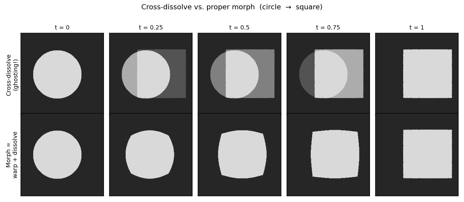
Top row: cross-dissolving a circle (left position) into a square (right position) — at every intermediate t you see two semi-transparent shapes, the classic ghost. Bottom row: a proper morph interpolates the geometry (position and shape) first and only then blends — one clean shape that really turns from circle into square. বাংলা: উপরের সারি: বৃত্ত থেকে বর্গে cross-dissolve — মাঝের প্রতিটা t-তে দুটো আধা-স্বচ্ছ আকৃতি একসাথে দেখা যায়, এটাই ghost। নিচের সারি: আসল morph — আগে geometry (অবস্থান + আকৃতি) interpolate, তারপর রঙ মেশানো — একটাই পরিষ্কার আকৃতি, সত্যি সত্যি বৃত্ত থেকে বর্গ হয়ে যাচ্ছে।
This is the whole chapter in one image. Same inputs, same blending weights \((1-t)\) and t — the only difference is whether the geometry was aligned before blending. Note where the ghost is worst: \(t = 0.5\), exactly as the \(t(1-t)\) factor of §4.10 predicts.
বাংলা: পুরো chapter-এর সারমর্ম এই এক ছবিতে। Input একই, blend-এর ওজনও একই — পার্থক্য শুধু একটাই: মেশানোর আগে geometry মেলানো হয়েছে কি না। আর ভূত কোথায় সবচেয়ে প্রকট দেখুন — t = 0.5-এ, ঠিক যেমনটা §4.10-এর \(t(1-t)\) factor বলে।
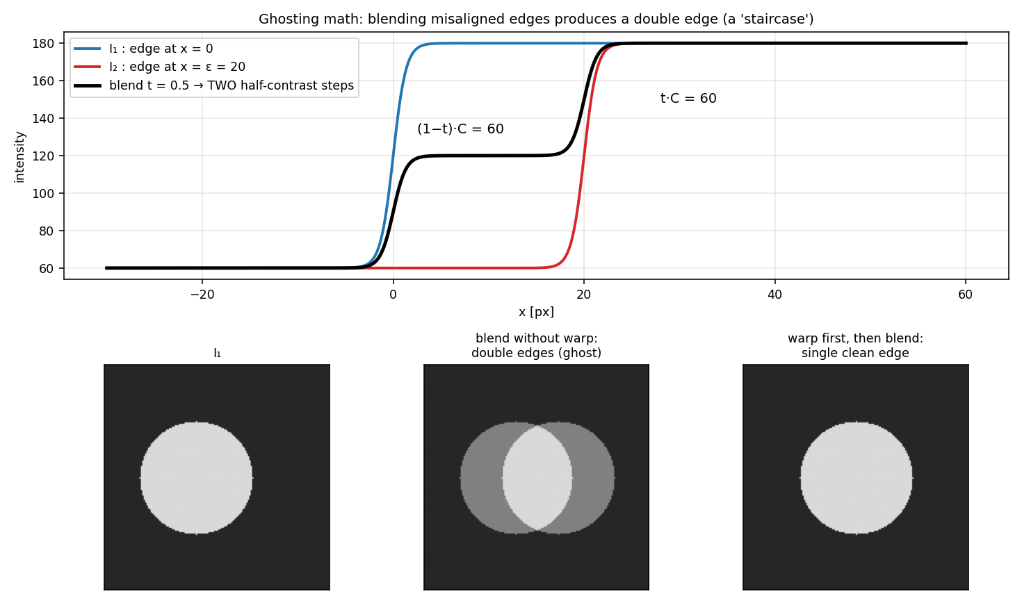
Top: two edges of contrast C = 120 misaligned by ε = 20 px; the t = 0.5 blend is a staircase with two half-contrast steps of 60 gray levels each — the 1-D anatomy of a ghost. Bottom: the same effect in 2-D — blending two shifted disks gives double edges, warping first gives one clean edge. বাংলা: উপরে: C = 120 contrast-এর দুটো edge, ε = 20 px misaligned; t = 0.5-এর blend একটা দুই-ধাপ সিঁড়ি — প্রতিটা ধাপ 60 gray level। এটাই ghost-এর 1-D ব্যবচ্ছেদ। নিচে: 2-D-তে একই জিনিস — সরে-থাকা দুটো চাকতি মেশালে জোড়া edge; আগে warp করলে একটাই পরিষ্কার edge।
Read the staircase against §4.1: step heights \((1-t)\cdot C\) and \(t\cdot C\), separation ε. Neither input contains a double edge — it is a pure blending artifact, and the only cure is removing ε (warping) before the blend.
বাংলা: সিঁড়িটা §4.1-এর সূত্র দিয়ে পড়ুন: ধাপের উচ্চতা \((1-t)\cdot C\) আর \(t\cdot C\), ফাঁক ε। জোড়া edge কোনো input-এই ছিল না — এ ভূত জন্মায় মেশানোর সময়েই; ওষুধ একটাই — মেশানোর আগে ε-কে warp করে শূন্য করা।
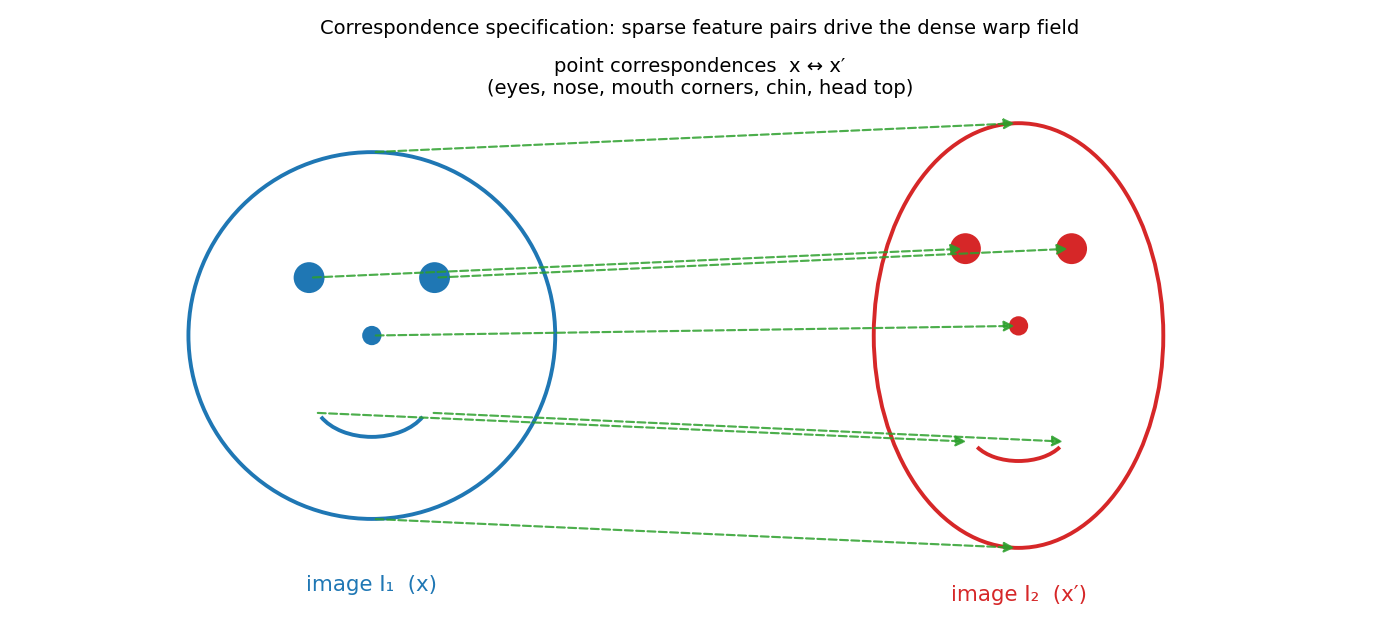
Two stylized faces — a small round one (I₁) and a tall narrow one (I₂) — with green dashed arrows pairing eyes, nose, mouth corners, chin, and head top: the sparse correspondences \(x \leftrightarrow x'\) a user clicks for a face morph. বাংলা: দুটো আঁকা মুখ — ছোট গোল (I₁) আর লম্বা সরু (I₂); সবুজ ড্যাশ-তীরগুলো চোখ, নাক, ঠোঁটের কোণ, থুতনি আর মাথার চূড়া জোড়া দিয়েছে — face morph-এর জন্য ব্যবহারকারীর ক্লিক-করা sparse correspondence \(x \leftrightarrow x'\)।
From these few anchors, scattered-data interpolation (triangulation, thin-plate splines, LWR — §2.7) spreads a displacement to every pixel: the dense warp field. Bad morphs are almost always traced back to this picture — too few, badly placed, or wrong pairs.
বাংলা: এই অল্প কটা নোঙর থেকেই scattered-data interpolation (triangulation, thin-plate spline, LWR — §2.7) প্রতিটা pixel-এর সরণ বানায় — সেটাই dense warp field। খারাপ morph-এর তদন্ত প্রায় সবসময় এই ছবিতেই এসে শেষ হয়: জোড়া কম, ভুল জায়গায়, বা ভুল।
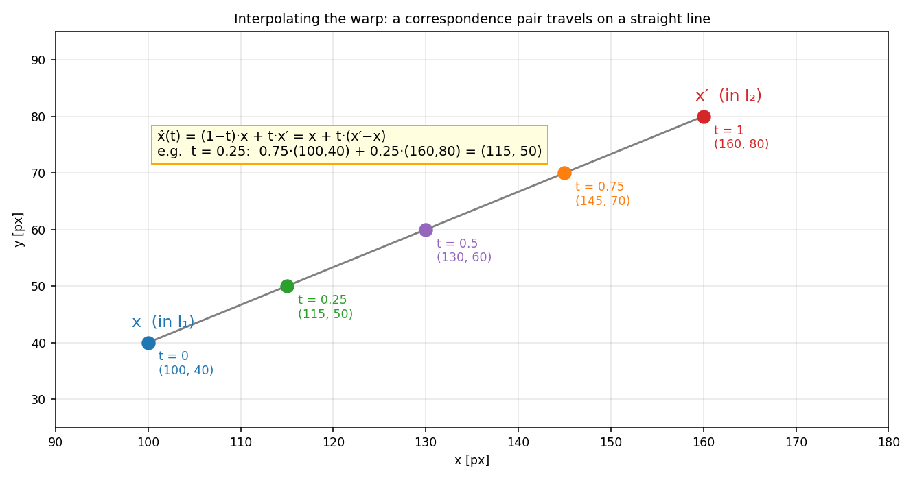
The correspondence pair x = (100, 40) ↔ x′ = (160, 80) travels on a straight image-space line at constant speed: t = 0.25 → (115, 50), t = 0.5 → (130, 60), t = 0.75 → (145, 70). বাংলা: Correspondence-জোড়া x = (100, 40) ↔ x′ = (160, 80) সরলরেখা ধরে সমান গতিতে হাঁটে: t = 0.25-এ (115, 50), t = 0.5-এ (130, 60), t = 0.75-এ (145, 70)।
This is §4.3 drawn out: \(\hat{x}(t) = (1-t)\cdot x + t\cdot x'\). Every pair gets its own straight line; the warp field is these moving anchors densified. And remember the chapter's warning — straight in image space is not physically correct in general (§4.7); that is what view morphing fixes.
বাংলা: §4.3-এর ছবি-রূপ: \(\hat{x}(t) = (1-t)\cdot x + t\cdot x'\) — প্রতিটা জোড়ার নিজের সরলরেখা। কিন্তু মনে রাখুন: image space-এ সরলরেখা মানেই physically সঠিক নয় (§4.7) — সেই ভুলটাই view morphing শোধরায়।
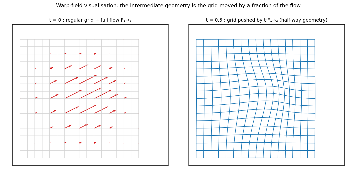
Left: a regular grid with the full flow F₁→₂ drawn as red arrows (a smooth bump pushing the center right-and-down-ish). Right: the same grid displaced by t·F₁→₂ at t = 0.5 — the half-way geometry every intermediate frame must show. বাংলা: বাঁয়ে: নিয়মিত grid-এর উপর পুরো flow F₁→₂ লাল তীরে আঁকা (মাঝখানে একটা মসৃণ ধাক্কা)। ডানে: একই grid t·F₁→₂ দিয়ে সরানো, t = 0.5 — মাঝপথের geometry, যেটা প্রতিটা intermediate frame-কে দেখাতে হবে।
"Warping by the scaled flow" is literally this: take the field, multiply by t, move the grid. At t = 0 the grid is untouched, at t = 1 it carries the full deformation — exactly the \(t\cdot F_{1}\to _{2}\) term in the morphing formula of §4.4.
বাংলা: "Scaled flow দিয়ে warp" মানে আক্ষরিকভাবেই এটা: field-টাকে t দিয়ে গুণ করে grid-টা সরাও। t = 0-তে grid অক্ষত, t = 1-এ পুরো বিকৃতি — §4.4-এর সূত্রের \(t\cdot F_{1}\to _{2}\) পদটা ঠিক এই কাজই করে।
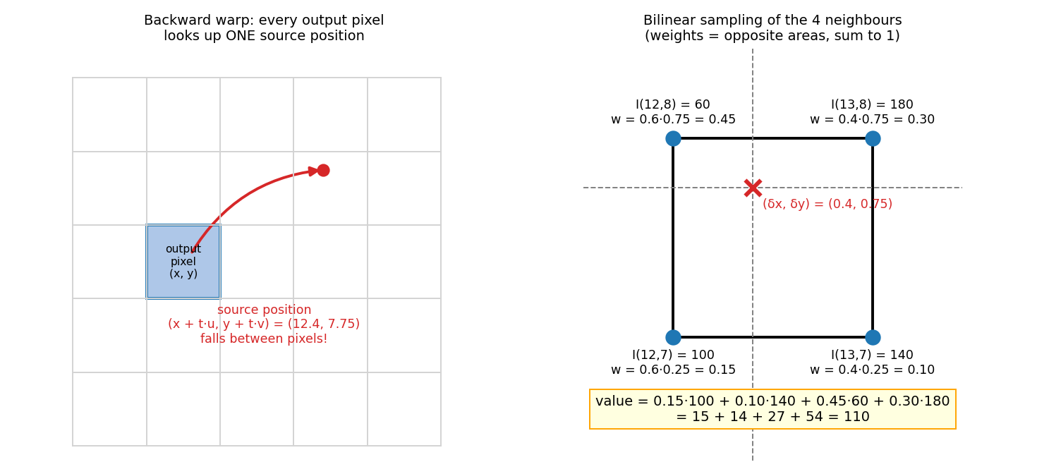
Left: backward warping — each output pixel looks up one source position (x + t·u, y + t·v) = (12.4, 7.75), which falls between pixels. Right: bilinear sampling of the 4 neighbors with the §4.5 numbers — weights 0.15, 0.10, 0.45, 0.30 (opposite areas, sum 1) and result 110. বাংলা: বাঁয়ে: backward warp — প্রতিটা output pixel একটাই উৎস-অবস্থান খোঁজে: (x + t·u, y + t·v) = (12.4, 7.75) — যা pixel-এর ফাঁকে পড়ে। ডানে: চার প্রতিবেশীর bilinear sampling, §4.5-এর সংখ্যা সমেত — ওজন 0.15, 0.10, 0.45, 0.30 (উল্টো দিকের ক্ষেত্রফল, যোগফল 1), ফল 110।
This is the Chapter-7 machinery the morph reuses for every single warped pixel. The worked numbers in the figure are the exact ones from §4.5 and the mock exam — if you can reproduce this picture, the sampling question is free points.
বাংলা: Morph-এর প্রতিটা warped pixel-এ Ch 7-এর এই যন্ত্রটাই চলে। ছবির সংখ্যাগুলো §4.5 আর mock exam-এর হুবহু এক — এই ছবিটা আঁকতে পারলেই sampling-প্রশ্নের নম্বর ফ্রি।
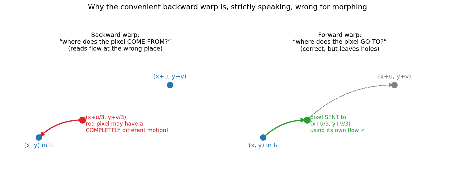
Left: backward warp asks "where does the pixel come from?" — but it reads the flow at the output location, where the resident pixel may have a completely different motion. Right: forward warp pushes each source pixel along its own scaled flow (correct), at the price of splatting and holes. বাংলা: বাঁয়ে: backward warp জিজ্ঞেস করে "pixel-টা কোথা থেকে আসে?" — কিন্তু flow পড়ে output জায়গায় বসে, যেখানকার pixel-এর গতি সম্পূর্ণ অন্যরকম হতে পারে। ডানে: forward warp প্রতিটা source pixel-কে তার নিজের scaled flow ধরে ঠেলে দেয় (সঠিক) — দাম: splatting আর গর্ত।
The lecture's subtle correctness point (§2.9, §4.6) in one picture. Memorize the two captions as exam vocabulary: backward = "come from" (convenient, hole-free, slightly wrong), forward = "go to" (correct, but splatting + holes).
বাংলা: Lecture-এর সূক্ষ্ম পয়েন্টটা (§2.9, §4.6) এক ছবিতে। দুটো বাক্য মুখস্থ রাখুন: backward = "কোথা থেকে আসে" (সুবিধাজনক, গর্তহীন, একটু ভুল); forward = "কোথায় যায়" (সঠিক, কিন্তু splatting + গর্ত)।
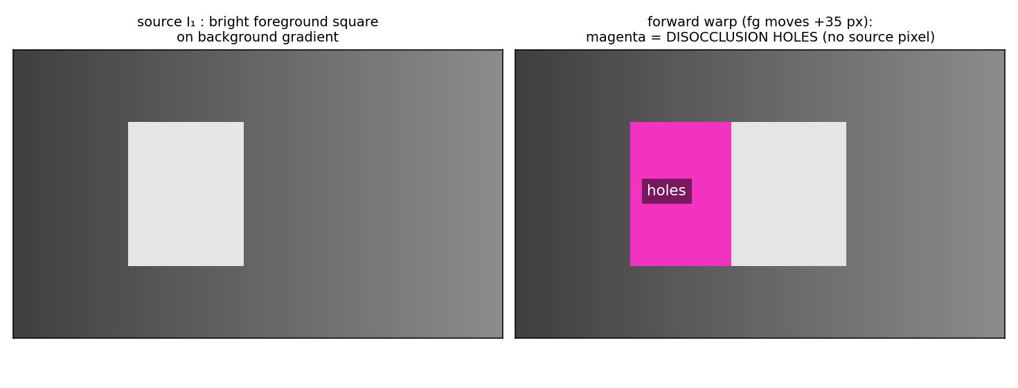
Left: source image — a bright foreground square on a background gradient. Right: after forward-warping the foreground +35 px to the right, the vacated strip is magenta — disocclusion holes where no source pixel lands, because the background there was never imaged. বাংলা: বাঁয়ে: source ছবি — background gradient-এর উপর উজ্জ্বল foreground বর্গ। ডানে: foreground-কে +35 px ডানে forward warp করার পর খালি-হওয়া ফালিটা magenta — disocclusion hole: ওখানে কোনো source pixel পড়ে না, কারণ ওই background অংশটা ক্যামেরা কখনো দেখেইনি।
This is the fundamental, not-fixable-by-better-flow limitation of §2.13: the information simply does not exist in I₁. Practical systems fill from the other image (if it sees the region), from the background, or by inpainting.
বাংলা: §2.13-এর মৌলিক সীমাবদ্ধতা — ভালো flow দিয়েও সারে না, কারণ তথ্যটাই I₁-এ নেই। বাস্তবে গর্ত ভরা হয় অন্য ছবি থেকে (যদি সে অঞ্চলটা দেখে), background থেকে, বা inpainting দিয়ে।
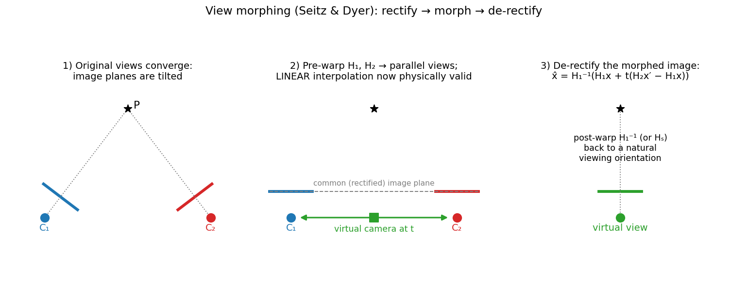
The Seitz & Dyer pipeline: 1) the original cameras C₁, C₂ converge on P with tilted image planes; 2) pre-warp with H₁, H₂ makes the views parallel with a common image plane — there, linear interpolation equals a real virtual camera at fraction t of the baseline; 3) post-warp (H₁⁻¹ or an interpolated Hₛ) returns the morphed image to a natural orientation. বাংলা: Seitz–Dyer pipeline: ১) আসল ক্যামেরা C₁, C₂ converging, image plane হেলানো; ২) H₁, H₂ দিয়ে pre-warp করলে view দুটো parallel হয়, image plane এক — ওখানে linear interpolation মানেই baseline-এর t ভগ্নাংশে দাঁড়ানো সত্যিকারের virtual ক্যামেরা; ৩) post-warp (H₁⁻¹ বা মাঝামাঝি Hₛ) দিয়ে ছবিটা স্বাভাবিক orientation-এ ফেরত।
Panel 2 is where the magic lives — the §4.8 proof applies only to parallel cameras, which is exactly what rectification manufactures. The formula under panel 3, \(\hat{x} = H_{1}^{-1}(H_{1}x + t(H_{2}x' - H_{1}x))\), is the trial-exam Q8a item.
বাংলা: জাদুটা প্যানেল ২-এ — §4.8-এর প্রমাণ কেবল parallel ক্যামেরায় খাটে, আর rectification ঠিক সেটাই বানিয়ে দেয়। প্যানেল ৩-এর নিচের সূত্র \(\hat{x} = H_{1}^{-1}(H_{1}x + t(H_{2}x' - H_{1}x))\) — এটাই trial exam-এর Q8a।
§6 Algorithms & Code¶
There is no dedicated exercise sheet for Chapter 9. The rectification (pre-warp) code lives in Ex/6/sheet6/epipolar_geometry.py (Chapter 8); feature matching comes from Chapter 5; dense flow from Chapter 6. The snippets below are the chapter's own algorithms, in the order of the pipeline.
6.1 Cross-dissolve¶
"""
Purpose: the baseline transition — pure color blend, no warp.
Input:   two equal-size images A, B; t in [0, 1].
"""
import numpy as np

def cross_dissolve(A, B, t):
    blend = (1 - t) * A.astype(np.float32) + t * B.astype(np.float32)
    return np.clip(blend, 0, 255).astype(np.uint8)

# frames = [cross_dissolve(A, B, t) for t in np.linspace(0, 1, 30)]
Step-by-step. Cast to float before blending (uint8 arithmetic would wrap around), form the convex combination, clip, cast back. One multiply-add per pixel — \(O(W\cdot H)\) per frame, the cheapest transition that exists.
Exam relevance. "Does cross-dissolve perform geometric alignment?" — No, and that is the whole point of the Q8c True/False item: it blends colors at fixed pixel positions, which is exactly why misaligned content ghosts (§4.1).
বাংলা: মেশানোর আগে float-এ cast জরুরি — uint8-এ \(0.75\cdot 200 + 0.25\cdot 80\) জাতীয় হিসাব মাঝপথে wrap করে যেতে পারে। আর পরীক্ষার মূল কথা: cross-dissolve-এ কোনো geometric alignment নেই — রঙ মেশে স্থির pixel-অবস্থানে, সেজন্যই ghost হয়।
6.2 Full morph with a dense flow field (backward-warp implementation)¶
"""
Purpose: the lecture's morphing formula
         I_M(t) = (1-t)·(t·F12 ∘ I1) + t·((1-t)·F21 ∘ I2)
Input:   I1, I2; dense fields f12, f21 of shape (H, W, 2); t in [0, 1].
"""
import cv2

def morph(I1, I2, f12, f21, t):
    h, w = I1.shape[:2]
    yy, xx = np.mgrid[0:h, 0:w].astype(np.float32)

    # warp I1 a fraction t along F1->2   (backward warp, bilinear)
    sx1 = xx + t * f12[..., 0]
    sy1 = yy + t * f12[..., 1]
    W1 = cv2.remap(I1, sx1, sy1, cv2.INTER_LINEAR)

    # warp I2 a fraction (1-t) along F2->1
    sx2 = xx + (1 - t) * f21[..., 0]
    sy2 = yy + (1 - t) * f21[..., 1]
    W2 = cv2.remap(I2, sx2, sy2, cv2.INTER_LINEAR)

    # cross-dissolve the two geometry-aligned images
    return cross_dissolve(W1, W2, t)
Step-by-step. Build the output pixel grid; add the t-scaled flow to get each source position (\(\hat{I}(x,y) = I(x + t\cdot u, y + t\cdot v)\) — §4.4); cv2.remap does the backward warp with bilinear sampling in one call (§4.5); finally blend with weights \((1-t)\), t. Note f21 is its own field anchored in I₂ — not -f12 pixelwise.
Failure cases. Backward warping reads the flow at the output position — wrong near motion discontinuities (§4.6); flow errors of size e produce ghosts of amplitude \(\approx t(1-t)\cdot \|e\|\cdot \|\nabla I\|\) (§4.10); disoccluded regions have no valid flow at all (§2.13).
বাংলা: তিন ধাপ: output grid বানাও; flow-কে t (এবং অন্য ছবিতে 1−t) দিয়ে স্কেল করে উৎস-অবস্থান বের করো; cv2.remap দিয়ে backward warp + bilinear, শেষে \((1-t)\), t ওজনে dissolve। সাবধান: f21 আলাদা field, pixel ধরে ধরে \(-f12\) নয়; আর object-এর কিনারায় backward warp-এর অনুমান ভাঙে।
6.3 Forward warp with splatting and hole detection¶
"""
Purpose: the 'strictly correct' warp of §4.6 — push each source pixel
         along ITS OWN scaled flow; mark holes where nothing lands.
"""
def forward_warp(I, f, t):
    h, w = I.shape[:2]
    out  = np.zeros_like(I, dtype=np.float32)
    wsum = np.zeros((h, w), dtype=np.float32)      # splat weight accumulator
    for y in range(h):
        for x in range(w):
            tx, ty = x + t * f[y, x, 0], y + t * f[y, x, 1]
            x0, y0 = int(np.floor(tx)), int(np.floor(ty))
            dx, dy = tx - x0, ty - y0
            for (xi, yi, wgt) in [(x0, y0, (1-dx)*(1-dy)), (x0+1, y0, dx*(1-dy)),
                                  (x0, y0+1, (1-dx)*dy),   (x0+1, y0+1, dx*dy)]:
                if 0 <= xi < w and 0 <= yi < h:
                    out[yi, xi]  += wgt * I[y, x]   # bilinear SPLAT
                    wsum[yi, xi] += wgt
    holes = wsum < 1e-3                             # disocclusion: nothing arrived
    out[~holes] /= wsum[~holes, None] if I.ndim == 3 else wsum[~holes]
    return out, holes
Step-by-step. Each source pixel computes its own non-integer target \((x + t\cdot u, y + t\cdot v)\) and distributes its value over the 4 surrounding output pixels with bilinear weights (splatting — the mirror image of bilinear sampling). Accumulated weights normalize the result; pixels where (almost) no weight arrived are holes — exactly the magenta strip of the §5 occlusion figure. A real implementation also resolves collisions by depth/visibility, vectorizes the loops, and fills the holes (other image / background / inpainting).
বাংলা: প্রতিটা source pixel নিজের flow ধরে ভগ্নাংশ-অবস্থানে যায় এবং চার প্রতিবেশী output pixel-এ ওজন অনুযায়ী নিজের মান ছড়িয়ে দেয় (splatting — bilinear sampling-এর আয়না-প্রতিবিম্ব)। যেখানে কিছুই এসে পড়ে না, সেটাই hole (disocclusion)। পূর্ণাঙ্গ বাস্তবায়নে সংঘর্ষ মেটাতে depth লাগে আর গর্ত ভরতে হয় আলাদা করে।
6.4 Triangulation morph (Delaunay + piecewise affine)¶
"""
Purpose: point-correspondence morphing à la 3dthis.com —
         Delaunay-triangulate, warp each triangle affinely, blend.
Input:   point arrays PA, PB of shape (N, 2); images A, B; t.
"""
def triangle_morph(A, B, PA, PB, tris, t):
    Pt  = (1 - t) * PA + t * PB                  # interpolated anchor points
    out = np.zeros_like(A, dtype=np.float32)
    for tri in tris:                             # tri = 3 point indices
        Ma = cv2.getAffineTransform(PA[tri].astype(np.float32),
                                    Pt[tri].astype(np.float32))
        Mb = cv2.getAffineTransform(PB[tri].astype(np.float32),
                                    Pt[tri].astype(np.float32))
        wa = cv2.warpAffine(A, Ma, A.shape[1::-1])
        wb = cv2.warpAffine(B, Mb, B.shape[1::-1])
        mask = np.zeros(A.shape[:2], np.uint8)
        cv2.fillConvexPoly(mask, np.int32(Pt[tri]), 1)
        out[mask > 0] = ((1 - t) * wa + t * wb)[mask > 0]
    return out.astype(np.uint8)
Step-by-step. Interpolate the clicked anchor points (§4.3); for every Delaunay triangle, the three moved vertices define one affine map per source image; warp both images, blend with \((1-t)\), t inside that triangle only. Piecewise-affine = continuous overall, linear inside each triangle. This is the densification-by-triangulation option of §2.7.
বাংলা: নোঙর-বিন্দুগুলো আগে interpolate হয়; প্রতিটা Delaunay ত্রিভুজের তিনটা সরে-যাওয়া শীর্ষ একটা করে affine map ঠিক করে দেয়; ত্রিভুজের ভেতরে warp + blend। টুকরো-টুকরো affine — পুরো ছবিতে continuous, প্রতিটা ত্রিভুজে linear। এটাই §2.7-এর triangulation densification।
6.5 View morphing — the Q8a formula in code¶
"""
Purpose: physically valid morph of one correspondence pair
         x_hat = H1^-1 (H1 x + t (H2 x' - H1 x)).
Input:   homogeneous 3-vectors x, xp; homographies H1, H2; t.
"""
def view_morph_point(x, xp, H1, H2, t):
    r1 = H1 @ x;   r1 = r1 / r1[2]      # rectify x        (dehomogenize!)
    r2 = H2 @ xp;  r2 = r2 / r2[2]      # rectify x'
    r  = r1 + t * (r2 - r1)             # linear interp in rectified frame
    xh = np.linalg.inv(H1) @ r          # de-rectify into image-1 frame
    return xh / xh[2]
Step-by-step. Rectify both points (and dehomogenize — divide by the third coordinate — before interpolating, otherwise the straight line is wrong); walk a fraction t from \(H_{1}x\) toward \(H_{2}x'\); map back with \(H_{1}^{-1}\). For whole images, prefer warping the coordinates like this and sampling colors from the originals once — one resampling instead of two, hence sharper (§2.11).
Sanity check. \(H1 = H2 = np.eye(3)\) collapses the function to plain \(x + t\cdot (x' - x)\) — the physically invalid image-space interpolation. The rectification round-trip is the entire added value.
বাংলা: তিন লাইনের অনুবাদ: rectify (তৃতীয় উপাদান দিয়ে ভাগ করতে ভুলবেন না!), rectified frame-এ t ভগ্নাংশ হাঁটা, \(H_{1}^{-1}\) দিয়ে ফেরত। পুরো ছবির জন্য স্থানাঙ্ক warp করে আসল ছবি থেকে একবারই রঙ পড়া ভালো — resampling যত কম, ছবি তত ধারালো। আর \(H_{1} = H_{2} = \mathbf{I}\) বসালে এটা সাধারণ (ভুল) interpolation-এ নেমে আসে — পুরো লাভটাই rectification-এ।
6.6 Sand & Teller dissimilarity and best-frame search¶
"""
Purpose: temporal alignment of two videos — D(i,j) = lam*p^2 + m^2.
Input:   matched feature arrays X1, X2 of shape (N, 2) for a frame pair.
"""
def dissimilarity(X1, X2, lam=1.0):
    m = np.linalg.norm(X2 - X1, axis=1).mean()        # motion magnitude
    p = 0.0                                            # parallax: distance changes
    n = 0
    for a in range(len(X1)):
        for b in range(a + 1, len(X1)):
            d1 = np.linalg.norm(X1[a] - X1[b])
            d2 = np.linalg.norm(X2[a] - X2[b])
            p += abs(d2 - d1); n += 1
    p /= max(n, 1)
    return lam * p**2 + m**2

# best temporal match for frame i:  j* = argmin_j dissimilarity(features(i, j))
# found with an adaptive search along the roughly diagonal path in the (i, j) table
Step-by-step. m is the mean displacement of the matches (how far the content moved); p averages the change of pairwise distances between features (non-zero only if the viewpoint differs — parallax). Minimize D over j for each i; the adaptive (roughly diagonal, depth-first) search avoids the \(O(N^{2})\) full table. Reproduces the §4.9 worked example: matches (20,20)→(22,21), (30,40)→(33,42) give m ≈ 2.921, p ≈ 1.346, D ≈ 10.344 at λ = 1.
বাংলা: m = match-গুলোর গড় সরণ, p = feature-জোড়াদের পারস্পরিক দূরত্বের গড় পরিবর্তন (viewpoint বদলালেই কেবল বদলায়)। প্রতি i-এর জন্য D সর্বনিম্ন করা j-টাই সেরা match; পুরো টেবিল না ঘেঁটে কোণাকুণি adaptive search। §4.9-এর সংখ্যাগুলো এই code-ই দেয়: m ≈ 2.921, p ≈ 1.346, D ≈ 10.344।
§7 Trial-Exam Mapping¶
| Trial-exam item | What you must know | Where in this chapter |
|---|---|---|
| Q8a Explain the morphing formula \(\hat{x} = H_{1}^{-1}(H_{1}x + t\cdot (H_{2}x' - H_{1}x))\) | Rectify both points (H₁x, H₂x′), interpolate linearly in the rectified frame (physically valid there — parallel cameras), de-rectify with H₁⁻¹ | §2.11, §4.8, view-morph figure |
| Q8b How does rectification help in stereo image processing? | Common image plane parallel to the baseline → correspondences on the same scan-line → 1-D search, disparity \(d = x_{L} - x_{R}\); the same homographies make morphing physically valid | §2.11, §4.8 (+ Chapter 8) |
| Q8c Three True/False | Feature-based matching does work for video (Sand & Teller); cross-dissolve has no geometric alignment; physically valid morphs do require rectified views | §2.2–2.5, §2.10–2.11, §4.1, §4.7–4.8 |
Model answer (Q8a). "x is a pixel in image 1 and x′ its correspondence in image 2; H₁ and H₂ are the rectifying homographies. H₁x and H₂x′ map both points into the common rectified image plane. There, H₁x + t·(H₂x′ − H₁x) walks linearly from H₁x (t = 0) to H₂x′ (t = 1); because rectified views behave like parallel cameras, this linear walk is exactly the projection seen by a real camera at fraction t of the baseline — i.e. it is physically valid. Finally H₁⁻¹ maps the interpolated point back into the original frame of image 1, where the colors are looked up."
Model answer (Q8b). "Rectification re-projects both images onto a common image plane parallel to the baseline. Corresponding points then lie on the same scan-line (epipolar lines become horizontal image rows), so the correspondence search drops from 2-D to 1-D, disparity is simply d = x_L − x_R, and row-based stereo algorithms (block matching, dynamic programming, graph cuts) become efficient. View morphing exploits the same homographies: linear interpolation in the rectified views is physically valid."
Q8c answers with one-line reasons:
| Statement | Answer | Why |
|---|---|---|
| "Feature-based matching does not work for video sequences." | F | Sand & Teller's video matching is feature-based and works precisely on videos. |
| "Cross-dissolve simply blends images without geometric alignment." | T | \(M(t) = (1-t)I_{1} + t\cdot I_{2}\) — no warp anywhere. |
| "Physically valid morphs require view rectification." | T | Seitz & Dyer: image-space interpolation is generally invalid; rectify-interpolate-derectify is valid. |
The fully graded answers are in CVML_Trial_Exam_Analysis.md.
§8 Mock Exam — 20 Questions¶
Answer everything on paper first; full worked solutions follow in §8.5. Tier A = basics, B = intuition, C = harder computation/derivation, D = transfer questions slightly beyond the lecture (typical for a tough oral or a "Transfer" section in the written exam).
Tier A — Basic (definitions & direct formula use)¶
A1. Write down the cross-dissolve formula. What exactly do you see at t = 0 and t = 1? Then compute the blended gray value for \(I_{1} = 180\), \(I_{2} = 60\) at \(t = 0.25\).
A2. Name the two ingredients of a morph and state why they must run in sync over t. What do you get if you keep only ingredient 2?
A3. State the view-morphing formula and name every symbol in it (x, x′, H₁, H₂, t, x̂).
A4. Define forward warping and backward warping in one sentence each (the "go to" / "come from" phrasing counts). Which of the two leaves holes, and which is the standard convenient choice?
A5. Write Sand & Teller's frame dissimilarity D(i, j) and explain in one sentence each what p, m, and \(\operatorname{argmin}_{j} D(i, j)\) mean.
Tier B — Intuitive (why / when)¶
B6. Why does a cross-dissolve of two misaligned images show double edges, and why is the effect worst around t = 0.5? Argue with the step-edge model.
B7. Even with perfect dense correspondences, plain image-space morphing of two photos of a static scene is physically invalid. Why? (One sentence about perspective projection suffices — plus the bent-plate symptom.)
B8. Why does rectifying the two views make linear interpolation physically valid? What property of the rectified camera pair does the §4.8 proof actually use?
B9. The lecture calls backward warping "strictly speaking not correct" for morphing. Explain the exact flaw, state when the approximation is harmless, and where it breaks.
B10. In the Virtual Video Camera, why are the recorded frames arranged in a space-time cube that is then tetrahedralized, and what goes wrong with a naive tetrahedralization when you move the virtual camera purely along the time axis?
Tier C — Harder (multi-step computation / derivation)¶
C11. Cross-dissolve an RGB pixel at \(\alpha = 0.6\): \(I_{0} = (40, 200, 120)\), \(I_{1} = (240, 100, 20)\) with \(M = (1-\alpha )\cdot I_{0} + \alpha \cdot I_{1}\). Compute all three channels, and state (with reason) the largest value any channel could ever reach during the whole transition α ∈ [0, 1].
C12. Two correspondences are given: \(P: (40, 60) \to (80, 100)\) and \(Q: (120, 20) \to (100, 60)\). (a) Compute the morphed positions of P and Q at \(t = 0.25\) and \(t = 0.5\). (b) Compute the distance ‖Q − P‖ in I₁, in I₂, and between the morphed points at t = 0.5 — does the distance interpolate linearly? What does that tell you?
C13. One full warp-and-blend output pixel: \(t = 0.25\), output position (8, 6), fields \(F_{1}\to _{2}(8, 6) = (4, 8)\) and \(F_{2}\to _{1}(8, 6) = (-4, -8)\), images \(I_{1}(9, 8) = 200\), \(I_{2}(5, 0) = 120\). Using the backward-warp morph of §4.4, compute both source positions and the final blended value.
C14. A backward warp requests the source position (4.2, 9.6). The four neighbors are \(I(4,9) = 50\), \(I(5,9) = 90\), \(I(4,10) = 110\), \(I(5,10) = 150\). Compute the four bilinear weights (show they sum to 1) and the sampled value.
C15. View morphing by hand: \(H_{1}\) translates by \((-10, 0)\), \(H_{2}\) translates by \((+20, -10)\); \(x = (40, 30, 1)^{T}\), \(x' = (90, 70, 1)^{T}\), \(t = 0.4\). (a) Compute \(H_{1}x\), \(H_{2}x'\), the interpolated rectified point, and x̂. (b) Compare with the naive image-space interpolation \(x + t(x' - x)\) and explain why the two answers differing matters.
Tier D — Transfer (adjacent to, but beyond, the lecture)¶
D16. Seitz & Dyer's view morphing vs plain morphing: under what camera configuration is plain image-space morphing of a static scene accidentally physically valid even without rectification? What extra information does view morphing need before it can run, and name two scene/timing assumptions under which even view morphing stops being valid.
D17. Beier–Neely line-based morphing weights each line pair's suggested displacement by \(w = (L^{p} / (a + d))^{b}\), where d is the pixel's distance to the line, L the line length, and a, b, p user constants. (a) Explain the roles of a, b, and p. (b) A pixel receives displacement suggestions (4, 0) from line 1 (d = 2) and (0, 4) from line 2 (d = 8). With \(p = 0, b = 1, a = 1\), compute the normalized weights and the blended displacement. © Why lines instead of points?
D18. Compare flow-based morphing (dense field from optical flow / FlowNet 2.0) with feature-based morphing (user-clicked points/lines): for each, name the input cost, the class of image pairs it can handle, and its characteristic failure mode. Which would you pick for (i) two consecutive video frames, (ii) a face-to-tiger morph — and why?
D19. The plenoptic function \(P(x, y, z, \theta , \phi , \lambda , t)\) describes all light in a scene. (a) What does each argument mean, and how many dimensions survive for a static scene at one wavelength? (b) Why can the 5-D version be reduced to a 4-D light field in free space? © Explain in two sentences how light-field rendering generalizes this chapter's view interpolation, and where view morphing sits inside that picture.
D20. Modern TVs offer "motion smoothing": they synthesize intermediate frames between broadcast frames (motion-compensated frame interpolation — exactly this chapter's morphing with automatically estimated flow). Using the chapter's theory, explain (a) why halo/ghosting artifacts cluster around the edges of fast-moving objects, (b) why artifacts are strongest in the synthesized frame half-way between two originals, and © why a pure cross-dissolve interpolator would look even worse ("soap-opera effect" aside).
§8.5 Solutions¶
Tier A¶
A1. \(M(t) = (1 - t)\cdot I_{1} + t\cdot I_{2}\), t ∈ [0, 1]. At t = 0 you see exactly I₁, at t = 1 exactly I₂ (the weights are (1, 0) and (0, 1)).
বাংলা: Cross-dissolve = convex combination; t = 0-তে পুরো I₁, t = 1-এ পুরো I₂ — মাঝে শুধু রঙের ভাগাভাগি: 0.75·180 + 0.25·60 = 150।
A2. (1) Geometric warp — both images are distorted so corresponding structures overlap at the intermediate geometry of time t; (2) cross-dissolve — the warped colors are blended with weights (1−t), t. They must share the same t: the color blend only looks right if the geometry shown by both images is already identical at that instant. Keeping only ingredient 2 gives the plain cross-dissolve — ghosting on any misaligned content.
বাংলা: Morph = warp + dissolve, দুটোই একই t-র তালে — geometry আগে এক না করলে রঙ মেশানো মানেই ভূত। শুধু dissolve রাখলে যা পাবেন তার নাম cross-dissolve।
A3. \(\hat{x} = H_{1}^{-1}\cdot (H_{1}x + t\cdot (H_{2}x' - H_{1}x))\). x = pixel in image 1 (homogeneous); x′ = its correspondence in image 2; H₁, H₂ = the rectifying homographies mapping each view onto the common plane parallel to the baseline; t ∈ [0, 1] = position of the virtual camera along the baseline; x̂ = the morphed position expressed back in image-1 coordinates (after de-rectification by H₁⁻¹).
বাংলা: সূত্রের তিন ধাপ মুখস্থ: rectify (H₁x, H₂x′) → rectified frame-এ t দিয়ে সোজা হাঁটা → H₁⁻¹ দিয়ে ফেরত; t মানে baseline-এ virtual ক্যামেরার অবস্থান।
A4. Backward warping: for every output pixel, ask "where does it come from?" and pull the value from \((x + t\cdot u, y + t\cdot v)\). Forward warping: for every source pixel, ask "where does it go to?" and push it there. Forward leaves holes (disocclusion: positions where no source pixel lands); backward is the standard convenient choice because every output pixel is guaranteed a value.
বাংলা: Backward = "কোথা থেকে আসে" (সুবিধাজনক, গর্তহীন); forward = "কোথায় যায়" (সঠিক কিন্তু গর্ত + splatting)।
A5.
\(D(i, j) = \lambda \cdot p^{2}(i, j) + m^{2}(i, j)\). p (parallax similarity) = how much the pairwise distances between matched features changed between the frames — non-zero only if the viewpoints differ. m (motion magnitude) = mean pixel displacement of the matched features — how far the content shifted overall. \(\operatorname{argmin}_{j} D(i, j)\) = the frame of video 2 that best matches frame i of video 1 (the temporal alignment).
বাংলা: p = feature-দের পারস্পরিক দূরত্বের বদল (viewpoint-এর সাক্ষী), m = গড় সরণ; D সর্বনিম্ন যেখানে, সেই j-ই frame i-এর সেরা জোড়া।
Tier B¶
B6. Model the misaligned edge: I₁ has an edge of contrast C at position a, I₂ has the same edge at a + ε. The blend \(B + C\cdot [(1-t)\cdot u(x-a) + t\cdot u(x-a-\epsilon )]\) is a staircase with two steps — height \((1-t)\cdot C\) at a and \(t\cdot C\) at a + ε. Neither input contains a double edge, so the eye reads it as a semi-transparent ghost. Around t = 0.5 both steps have height C/2 — both copies are equally strong, neither dominates, so the artifact is maximally visible; near t = 0 or 1 one copy fades toward zero contrast. (Quantitatively the ghost scales with t(1−t), §4.10.)
বাংলা: Misaligned edge মেশালে দুই-ধাপ সিঁড়ি — উচ্চতা (1−t)·C আর t·C; t = 0.5-এ দুটোই C/2, তাই তখনই ভূত সবচেয়ে স্পষ্ট।
B7. Perspective projection divides by depth (\(p = f\cdot X/Z\)), so it is non-linear in the 3-D point — the projection of a 3-D midpoint is not the midpoint of the projections. Image-space morphing assumes exactly that equality, point by point, so each surface point lands at a differently-wrong position; on a rigid flat plate the intermediate frames show the plate bending — an image no real camera could capture. Perfect correspondences fix which points are paired, not where the linear path puts them.
বাংলা: Projection depth দিয়ে ভাগ করে বলে non-linear — "গড়ের ছবি ≠ ছবির গড়"। তাই নিখুঁত correspondence থাকলেও সরল image-space interpolation-এ সমতল প্লেটও মাঝপথে বেঁকে যায়।
B8. Rectification re-projects both images onto a common plane parallel to the baseline — afterwards the two views behave like parallel cameras: same image plane, same f, centers differing only along the baseline, \(C_{s} = (s\cdot b, 0, 0)\). The §4.8 proof uses exactly this: the projection \(x_{s} = f\cdot (X - s\cdot b)/Z\) is linear in s (Z is the same for all s because the image plane doesn't rotate). Hence \((1-t)x_{0} + t\cdot x_{1} = f(X - t\cdot b)/Z\) — precisely what the real camera at fraction t of the baseline sees. The proof needs nothing else; that is why manufacturing parallelism (rectifying) is sufficient.
বাংলা: Rectified মানে parallel ক্যামেরা, আর তখন projection-টা s-এ linear: \(x_{s} = f(X - s\cdot b)/Z\) — তাই দুই প্রান্তের linear interpolation হুবহু মাঝের বাস্তব ক্যামেরার ছবি।
B9. The flow vector stored at (x, y) describes the motion of the scene point imaged at (x, y) in the source image. The backward warp \(\hat{I}(x, y) = I(x + t\cdot u(x,y), y + t\cdot v(x,y))\) evaluates the flow at the output location — i.e. it borrows the motion of whatever pixel starts there and applies it to the pixel that should arrive there, which "could have a completely different motion". Harmless wherever the flow field is smooth (\(F(x + t\cdot u) \approx F(x)\)); breaks at motion discontinuities — object boundaries — exactly where ghosts and bleeding appear and where user-defined correspondences are added.
বাংলা: Backward warp flow পড়ে ভুল জায়গায় — output-এ বসা pixel-এর গতি ধার করে। মসৃণ flow-তে ক্ষতি নেই; object-এর কিনারায় (motion discontinuity) ভুলটা ফুটে ওঠে।
B10. Each recorded frame is one vertex of a 3-D navigation space: two axes of camera position in the camera plane + one axis of time. Tetrahedralizing the cube gives, for any interior (position, time) query, exactly 4 enclosing vertex frames to morph between (with barycentric weights) — the minimal interpolation cell in 3-D. With a naive tetrahedralization, a query path that moves only along the time axis keeps crossing tetrahedra whose vertices belong to different camera subsets — the virtual camera appears to wobble although the requested position never moved. The tetrahedralization must therefore be chosen so that time-only motion reuses the same cameras.
বাংলা: Space-time cube-এ প্রতিটা ভেতরের বিন্দুর জন্য ৪টা ঘেরা-vertex-frame লাগে — তাই tetrahedron। যেনতেন ভাগ করলে শুধু সময়ে এগোলেও camera-set বদলে বদলে যায় — virtual ক্যামেরা কাঁপে।
Tier C¶
C11. Weights: \(1 - \alpha = 0.4\), \(\alpha = 0.6\).
R: 0.4·40  + 0.6·240 =  16 + 144 = 160
G: 0.4·200 + 0.6·100 =  80 +  60 = 140
B: 0.4·120 + 0.6·20  =  48 +  12 =  60

M(0.6) = (160, 140, 60)
Largest possible value during the whole transition: the blend is a convex combination (non-negative weights summing to 1), so no channel can ever exceed the larger of its two endpoints. The maximum over all channels and all α is therefore \(\max (240, 200, 120) = 240\) — attained by the R channel at α = 1.
বাংলা: Convex combination কখনো প্রান্তের বাইরে যায় না — তাই পুরো transition-এ সর্বোচ্চ মান হবে endpoint-দের সর্বোচ্চ, এখানে R-এর 240 (α = 1-এ)। আর α = 0.6-এ ফল (160, 140, 60)।
C12. (a) \(\hat{x}(t) = (1-t)\cdot x + t\cdot x'\) per pair:
P: t = 0.25: 0.75·(40, 60) + 0.25·(80, 100) = (30+20, 45+25) = (50, 70)
   t = 0.5 : (60, 80)
Q: t = 0.25: 0.75·(120, 20) + 0.25·(100, 60) = (90+25, 15+15) = (115, 30)
   t = 0.5 : (110, 40)
(b) Distances:
The linear average of the endpoint distances would be \((89.44 + 44.72)/2 = 67.08 \neq 64.03\). Positions interpolate linearly, distances do not (they only would if both points carried the same displacement, i.e. pure translation). Lesson: linear morphing preserves nothing about relative geometry — and a changing inter-feature distance is exactly what Sand & Teller's parallax term p detects.
বাংলা: বিন্দুর অবস্থান সরলরেখায় হাঁটে, কিন্তু দুই বিন্দুর দূরত্ব linear ভাবে বদলায় না (64.03 ≠ 67.08) — displacement দুটো আলাদা বলেই। এই দূরত্ব-বদলই Sand–Teller-এর p-এর খোরাক।
C13.
Step 1 — warp I₁ by t·F₁→₂:
  source₁ = (8 + 0.25·4 , 6 + 0.25·8) = (9, 8)        → Î₁(8, 6) = I₁(9, 8) = 200

Step 2 — warp I₂ by (1−t)·F₂→₁:
  source₂ = (8 + 0.75·(−4) , 6 + 0.75·(−8)) = (5, 0)  → Î₂(8, 6) = I₂(5, 0) = 120

Step 3 — blend with weights (1−t, t) = (0.75, 0.25):
  I_M(8, 6) = 0.75·200 + 0.25·120 = 150 + 30 = 180
Both source positions happen to be integer here; otherwise each lookup would be a bilinear sample (C14).
বাংলা: I₁ এগোয় t = ¼ ভগ্নাংশ, I₂ পেছায় ¾ ভগ্নাংশ — উৎস (9,8) আর (5,0); তারপর 0.75·200 + 0.25·120 = 180। ক্রমটা মুখস্থ: আগে দুই warp, পরে এক blend।
C14. \(x_{0} = 4, y_{0} = 9, \delta x = 0.2, \delta y = 0.6\):
w₀₀ = (1−0.2)(1−0.6) = 0.8·0.4 = 0.32      w₁₀ = 0.2·0.4 = 0.08
w₀₁ = 0.8·0.6        = 0.48               w₁₁ = 0.2·0.6 = 0.12
sum = 0.32 + 0.08 + 0.48 + 0.12 = 1.00 ✓

I(4.2, 9.6) = 0.32·50 + 0.08·90 + 0.48·110 + 0.12·150
            = 16 + 7.2 + 52.8 + 18 = 94
বাংলা: ওজন = উল্টো দিকের উপ-আয়তক্ষেত্রের ক্ষেত্রফল, যোগফল 1; এখানে ফল 94। δy = 0.6 মানে নিচের সারির (y = 10) ওজন বেশি — sanity check হিসেবে মিলিয়ে নিন।
C15. (a) Pure translations act on the first two homogeneous coordinates:
H₁x  = (40 − 10, 30 + 0, 1)  = (30, 30, 1)
H₂x′ = (90 + 20, 70 − 10, 1) = (110, 60, 1)

offset       = H₂x′ − H₁x = (80, 30, 0)
interpolated = (30, 30, 1) + 0.4·(80, 30, 0) = (62, 42, 1)
x̂            = H₁⁻¹·(62, 42, 1)ᵀ = (62 + 10, 42 − 0, 1) = (72, 42, 1)
(b) Naive image-space interpolation: \(x + 0.4\cdot (x' - x) = (40 + 0.4\cdot 50, 30 + 0.4\cdot 40) = (60, 46)\) — a different point (off by (12, −4)). The difference is the physical-validity correction: (72, 42) is where a real camera at 40% of the baseline would image the scene point; (60, 46) corresponds to no real camera at all (the bent-plate error, distributed over the whole image).
বাংলা: Rectify-ঘুরে-আসা উত্তর (72, 42), সরাসরি interpolation দিত (60, 46) — পার্থক্যটুকুই physics: প্রথমটা বাস্তব ক্যামেরার ছবি, দ্বিতীয়টা কারো নয়।
Tier D¶
D16. Plain morphing is accidentally valid when the two cameras are already in the rectified configuration — parallel image planes that are parallel to the baseline (e.g. a camera translated strictly sideways with no rotation, as in a standard parallel stereo rig): then H₁ = H₂ ≈ 𝐈 and the §4.8 proof applies directly to the raw images. (Equivalently: whenever the apparent 3-D motion of every point is parallel to the image plane, depth Z never changes and projection behaves linearly.) View morphing needs the rectifying homographies H₁, H₂ — i.e. the epipolar geometry / fundamental matrix from correspondences (Chapter 8) — before it can run. It stops being valid for dynamic scenes (the two photos are not two views of the same static geometry — e.g. the subject moved or the photos are of different people) and under visibility/appearance changes (occlusion differences, specular highlights that move with the light): then no single 3-D scene explains both images and the interpolated "camera" photographs nothing real.
বাংলা: ক্যামেরা আগে থেকেই parallel (পাশে-সরানো rig) হলে raw ছবিতেই morph valid — rectification তখন অপ্রয়োজনীয় formality। আর view morphing-ও ভাঙে যদি দৃশ্য static না হয় বা দুই ছবিতে visibility/specular বদলায় — তখন কোনো একক 3-D দৃশ্যই দুটো ছবি ব্যাখ্যা করে না।
D17.
(a) a — softening constant: it caps the weight as d → 0; with a ≈ 0, pixels on the line get (near-)infinite weight, i.e. the line is matched exactly; larger a makes the warp smoother but looser. b — locality exponent: how fast influence decays with distance; large b → each line only governs its neighborhood, small b → every line influences everything. p — length reward: p = 0 ignores line length; p > 0 gives longer lines more authority (a long jaw line should outvote a short eyebrow stroke).
(b) With p = 0, b = 1, a = 1: \(w = 1/(1 + d)\):
w₁ = 1/(1+2) = 1/3        w₂ = 1/(1+8) = 1/9
normalized:  w₁ = (1/3)/(1/3 + 1/9) = 3/4 = 0.75      w₂ = 1/4 = 0.25
displacement = 0.75·(4, 0) + 0.25·(0, 4) = (3, 1)
© A point pair fixes only a displacement at isolated dots; a line pair additionally fixes a local orientation and scale along a whole 1-D structure — exactly what facial features (eyebrows, jaw, hairline) are. That is why Beier–Neely produced the first convincing photorealistic face morphs (Black or White); its weak spot is curved edges, which lines only approximate.
বাংলা: a = রেখার ঠিক উপরে ওজন কত চড়বে (a→0 মানে রেখা হুবহু মানা হবে), b = প্রভাব কত দ্রুত দূরত্বে কমবে, p = লম্বা রেখার বাড়তি কর্তৃত্ব। হিসাব: ওজন ৩:১ → সরণ (3, 1)। রেখা বেছে নেওয়ার কারণ — সে orientation-ও বেঁধে দেয়, শুধু বিন্দু নয়।
D18.
| Flow-based | Feature-based | |
|---|---|---|
| Input cost | none (automatic: optical flow / FlowNet 2.0) | manual clicking of points/lines |
| Handles | related images: same scene / consecutive frames, small appearance gap (brightness constancy must roughly hold) | arbitrary, even unrelated images (face ↔ tiger) — the human supplies the semantics |
| Characteristic failure | flow is wrong at large displacements, occlusions, lighting changes → ghosts/tearing exactly at object boundaries | sparse coverage: anything between the clicked features deforms by interpolation, oddly if anchors are few/badly placed; labor does not scale |
(i) Two consecutive video frames: flow-based — brightness constancy holds, displacements are small, and clicking features per frame pair is absurd. (ii) Face-to-tiger: feature-based — no flow method can find correspondences between semantically different objects; the lecture's point that user-specified correspondences are required for unrelated images.
বাংলা: সম্পর্কিত ছবি (পরপর frame) → flow-based, ফ্রি আর dense; অসম্পর্কিত ছবি (মুখ ↔ বাঘ) → feature-based, কারণ correspondence-এর অর্থটা মানুষকেই দিতে হয় — কোনো network ওটা আন্দাজ করতে পারে না।
D19.
(a) (x, y, z) = the 3-D position of the observer/eye, \((\theta , \phi )\) = the viewing direction of the ray, \(\lambda\) = wavelength, t = time. A static scene drops t, one wavelength (or per-RGB-channel treatment) drops λ → a 5-D function of position and direction.
(b) In free space (no occluders between the measurement surfaces), radiance is constant along a ray — moving the observer along the ray changes nothing. One dimension is therefore redundant, and rays can be indexed by 4 numbers, e.g. their intersections (u, v) and (s, t) with two parallel planes: the 4-D light field (Lytro, camera arrays).
© Light-field rendering synthesizes any novel view by simply resampling stored rays — view interpolation with no correspondences and no geometry, provided the rays were sampled densely enough. This chapter's view morphing is the sparse extreme of the same idea: with only two cameras the ray database is far too sparse to resample, so the missing rays must be hallucinated via correspondences + rectified linear interpolation along the baseline.
বাংলা: Plenoptic = "কে, কোথা থেকে, কোন দিকে, কখন, কোন রঙের আলো দেখছে" — static+monochrome হলে 5-D, free space-এ ray-বরাবর radiance ধ্রুব বলে 4-D light field। Ray যথেষ্ট ঘন হলে নতুন view মানে শুধু resampling; মাত্র ২টা ক্যামেরা থাকলে সেই ঘাটতিটাই correspondence + view morphing দিয়ে পোষাতে হয়।
D20. (a) Motion-compensated interpolation is warp-then-blend with an automatically estimated flow. At the boundary of a fast-moving object the flow field is discontinuous and partly undefined: background pixels are disoccluded (no source data — holes to be filled) and the estimated flow inevitably bleeds across the boundary (the backward-warp flaw of §4.6). The resulting misplaced samples blend into translucent halos hugging exactly those edges. (b) By §4.10 the ghost amplitude scales with \(t(1-t)\cdot \|e\|\cdot \|\nabla I\|\): it vanishes at the original frames (t = 0, 1) and peaks at t = 0.5, where both warped images are furthest from their sources and neither copy dominates — so the synthesized middle frame is always the most fragile. © A pure cross-dissolve interpolator would skip motion compensation entirely: every moving edge would appear twice per synthesized frame, separated by the full inter-frame motion (ε = the entire displacement instead of just the flow error e) — uniform double-exposure ghosting far worse than localized halos. Motion compensation reduces the effective misalignment from the full motion to the flow error; the residual artifacts live where that error is largest — object boundaries.
বাংলা: TV-র frame interpolation এই chapter-এরই warp+blend — halo জমে object-এর কিনারায়, কারণ ওখানেই flow ভুল + disocclusion; মাঝের frame (t = 0.5) সবচেয়ে ভঙ্গুর \(t(1-t)\) factor-এর জন্য। আর খালি cross-dissolve করলে প্রতিটা চলন্ত edge পুরো গতি-দূরত্বে দু'বার ছাপা হতো — তার চেয়ে halo ঢের সহ্যযোগ্য।
§9 Exam-Day Cheat Sheet¶
The five formulas
Cross-dissolve:      M(t) = (1−t)·I₁ + t·I₂                       (no warp → ghosts)
Point interpolation: x̂(t) = (1−t)·x + t·x′ = x + t·(x′−x)
Full morph:          I_M(t) = (1−t)·(t·F₁→₂ ∘ I₁) + t·((1−t)·F₂→₁ ∘ I₂)
                     backward-warp term: Î(x,y) = I(x + t·u, y + t·v)  + bilinear
View morphing (Q8a): x̂ = H₁⁻¹·( H₁x + t·(H₂x′ − H₁x) )            rectify → interpolate → de-rectify
Video matching:      D(i,j) = λ·p² + m²       j* = argmin_j D(i,j)
Pipelines in one breath
- Morph = warp both images to the intermediate geometry (scaled flows t and 1−t), then cross-dissolve with (1−t), t. Endpoints check: t = 0 → I₁, t = 1 → I₂.
- View morphing (Seitz & Dyer) = pre-warp (rectify, H₁/H₂) → linear morph in the rectified frame → post-warp (H₁⁻¹ or interpolated Hₛ). Valid because rectified views = parallel cameras, where \(x_{s} = f(X - s\cdot b)/Z\) is linear in s — the interpolation IS a real camera on the baseline.
- Video matching (Sand & Teller) = features → match probabilities (Pᵢ pixel similarity · Mᵢ motion consistency via LWR) → dense field by LWR → warp; frame search by D(i,j) with adaptive ~diagonal walk.
- Virtual Video Camera = ~20 cameras → space-time cube (2 position axes + time) → tetrahedralize → morph the 4 enclosing vertex frames. Naive tetrahedralization → wobble on time-only paths. Bullet time for cheap.
Ghosting & errors
- Misaligned edge of contrast C → two steps: \((1-t)\cdot C\) at a, \(t\cdot C\) at a + ε. Worst at t = 0.5.
- Ghost amplitude ≈ \(t(1-t)\cdot \|e\|\cdot \|\nabla I\|\) — linear in flow error, scaled by image gradient, peaks mid-morph (factor ¼).
- Bilinear weights = opposite areas, sum to 1; drill numbers: (12.4, 7.75) with 100/140/60/180 → 110.
- Every resampling = mild low-pass ⇒ warp coordinates once (sharp) instead of images twice (blurry).
Physics or not?
- Projection divides by depth ⇒
project(mean P) ≠ mean(project P)⇒ image-space morphing bends rigid plates — physically invalid. - Exception: motion parallel to the image plane (Z constant) or cameras already parallel — then plain interpolation is already valid.
- Forward warp = correct ("go to", own flow; needs splatting, leaves holes). Backward warp = convenient ("come from"; reads flow at the wrong place; fine in smooth flow, wrong at motion discontinuities).
- Occlusion: no valid correspondence; disocclusion: holes — no 3-D info ⇒ fill from other image / background / inpainting. Speculars move with the light, not the surface.
Quick traps
- \(F_{2}\to _{1} \neq -F_{1}\to _{2}\) pixelwise — two different fields anchored in two different images.
- Dehomogenize (divide by 3rd coordinate) after applying H, before interpolating.
- \(H_{1} = H_{2} = \mathbf{I}\) collapses Q8a's formula to plain (invalid) interpolation — say it to show understanding.
- Distances between morphed points do NOT interpolate linearly — only positions do.
- Q8c: feature matching DOES work for video (F); cross-dissolve has NO alignment (T); physically valid ⇒ rectification (T).
বাংলা মন্ত্র (শেষ মুহূর্তের জপ)
- "Morph মানে warp + dissolve — আগে geometry, পরে রঙ; খালি dissolve মানেই ভূত, আর ভূতের রাজত্ব t = 0.5-এ।"
- "Q8a-র সূত্র তিন ধাপ: H দিয়ে rectified plane-এ যাও, t দিয়ে সোজা হাঁটো, H₁⁻¹ দিয়ে ফিরে এসো — মাঝের ছবিটা তখন সত্যিকারের ক্যামেরার।"
- "Projection depth দিয়ে ভাগ করে — তাই image-space morph-এ সোজা প্লেটও বেঁকে যায়; rectify করলে x_s হয় s-এ linear, আর সব বৈধ।"
- "Backward warp সুবিধার, forward warp সঠিক — forward-এর দাম splatting আর গর্ত, গর্তের নাম disocclusion।"
- "Sand–Teller: p মাপে viewpoint-এর ফারাক, m মাপে সরণ — D = λp² + m², সবচেয়ে কম D-ই জোড়া।"
- "যত নিখুঁত correspondence, তত পরিষ্কার morph — ভূতের মাপ t(1−t)·‖e‖·‖∇I‖।"
Final mantra: "Morph = warp + dissolve. Image-space morph is fake; rectify-then-interpolate is real. Backward asks where from, forward says where to. Cross-dissolve has NO geometric alignment. Feature-based matching DOES work for videos."