Chapter 02 — Filtering, Edges & Thresholding

Exam weight: 20 / 110 points — the HIGHEST-weight topic on the exam. The trial exam dedicates an entire question block to it, including a numerical convolution you must compute by hand. If you master only one chapter perfectly, make it this one.

বাংলা: এই chapter-টা পরীক্ষার সবচেয়ে গুরুত্বপূর্ণ অংশ — ১১০ নম্বরের মধ্যে ২০ নম্বর শুধু এখান থেকেই আসে। trial exam-এ হাতে-কলমে convolution হিসাব করতে হয়েছে, তাই এই chapter-এর প্রতিটা হিসাব নিজে হাতে করে অভ্যাস করো।

---

§1. Chapter Roadmap

This chapter covers everything needed to clean, enhance, and segment a single image:

1. Filtering — remove noise without destroying the signal (box, sinc, Gaussian, median).
2. Edges — find where intensity changes sharply (derivative filters, Sobel, Laplacian, LoG, DoG, Canny).
3. Thresholding — turn a gray image into a binary foreground/background mask (simple, Otsu, adaptive).

How the sections build on each other:

pixels → (noise!) → SMOOTHING filters → DERIVATIVE filters → gradient |∇I|, θ
       → Laplacian / LoG / DoG (2nd derivative) → Canny (the full edge pipeline)
       → histogram → thresholding (simple → Otsu → adaptive) → binary mask

Connections to other chapters:

• Chapter 4 (Machine Learning) — convolutional layers in CNNs are exactly the linear filters defined here.
• Chapter 5 (Features) — Harris uses Sobel gradients; SIFT uses DoG scale space.
• Chapter 6 (Optical Flow) — Lucas-Kanade needs spatial gradients I_x, I_y and Gaussian image pyramids.

Likely exam questions (taken from the trial exam):

• Match images to their Fourier power spectra.
• State the purpose of the Gaussian filter (short answer).
• State the purpose of DoG and what it approximates.
• Explain the difference between global and local thresholding.
• Remove a linear brightness gradient from a concrete-wall photo without destroying texture.
• Convolve a given 8×8 image with the kernel [-1, 0, 1] by hand.
• Identify a filter's category and name more filters of the same category.

বাংলা: এই chapter-এর গল্পটা এক লাইনে: ছবিতে noise থাকে, তাই আগে smoothing filter দিয়ে noise কমাই; তারপর derivative filter দিয়ে edge খুঁজি; শেষে threshold দিয়ে ছবিটাকে সাদা-কালো mask-এ ভাগ করি। পরীক্ষায় convolution হাতে হিসাব করা, Gaussian-এর উদ্দেশ্য বলা, DoG কী approximate করে, আর global vs local thresholding — এগুলো প্রায় নিশ্চিতভাবে আসবে।

---

§2. Concepts from Zero

2.1 What is a filter?

A filter is a small grid of numbers (called a kernel or mask, e.g. 3×3) that we slide over the image. At every position we multiply each kernel weight with the pixel underneath it and add everything up — the sum becomes one pixel of the output image. Different numbers in the kernel ⇒ completely different behaviour:

• Smoothing / blurring (noise removal): box, Gaussian, sinc, median.
• Edge detection: Prewitt, Sobel, Laplacian, LoG, DoG.
• Sharpening: unsharp masking.
• Feature extraction: Gabor wavelets, DoG (SIFT).

বাংলা: filter মানে একটা ছোট সংখ্যা-grid (kernel), যেটাকে ছবির ওপর slide করানো হয়। প্রতিটা জায়গায় kernel-এর সংখ্যাগুলো নিচের pixel-গুলোর সাথে গুণ করে সব যোগ করলে output ছবির একটা pixel পাওয়া যায়। kernel-এর সংখ্যা বদলালেই কাজ বদলে যায় — কখনো blur, কখনো edge detection, কখনো sharpening।

2.2 The true image function and sampling

A camera sensor samples a continuous 2-D function I(x, y) into discrete pixels. An image is therefore a sampled function, not just an array. Sampling loses information: by the Nyquist theorem, to capture a structure of frequency f you must sample with at least 2f — practically, the smallest visible feature must span at least 2 pixels. Sampling too coarsely creates aliasing: false low-frequency patterns (Moiré). That is why image pyramids always blur (Gaussian) before subsampling.

বাংলা: ছবি আসলে একটা continuous function-এর sample। Nyquist theorem বলে — কোনো structure ধরতে হলে তার frequency-র অন্তত দ্বিগুণ হারে sample নিতে হবে, মানে সবচেয়ে ছোট feature-ও যেন কমপক্ষে ২ pixel জুড়ে থাকে। তা না হলে aliasing হয় — ভুয়া প্যাটার্ন দেখা যায়। এই জন্যই image pyramid বানানোর আগে Gaussian blur করা বাধ্যতামূলক।

2.3 Frequencies in an image (Fourier view)

Any image can be decomposed into a weighted sum of 2-D sine/cosine waves of different frequency, amplitude, phase, and orientation (Fourier transform). The power spectrum (log-magnitude of the DFT, origin shifted to center) shows which frequencies are present:

• Smooth regions / slow illumination changes → low frequencies (near the center).
• Fine texture, sharp edges, noise → high frequencies (far from the center).
• Stripes in the image → two bright spots in the spectrum, perpendicular to the stripe direction.
• Rotating the image rotates the spectrum by the same angle.
• Convolution in image space = multiplication in Fourier space — the key theorem of this chapter.

বাংলা: যেকোনো ছবিকে সাইন-কোসাইন wave-এর যোগফল হিসেবে ভাবা যায়। ধীরে বদলানো অংশ (আলো, মসৃণ wall) = low frequency, আর ধারালো edge, texture, noise = high frequency। power spectrum-এ stripe-ওয়ালা ছবি দিলে stripe-এর সাথে লম্বভাবে (perpendicular) উজ্জ্বল বিন্দু দেখা যায়। সবচেয়ে দরকারি নিয়ম: image-এ convolution করা মানে Fourier domain-এ গুণ করা।

2.4 Noise and why we smooth

Real images contain noise (photon shot noise, sensor read noise, salt-and-pepper from dead pixels). Noise is mostly high-frequency. Smoothing filters average each pixel with its neighbours, which cancels zero-mean noise but unfortunately also blurs real edges — the eternal trade-off. Hybrid images are a fun demonstration of the frequency split: low frequencies of image A + high frequencies of image B look like B up close and A from far away.

বাংলা: আসল ছবিতে সবসময় noise থাকে, আর noise মূলত high-frequency। smoothing filter প্রতিবেশী pixel-দের গড় নেয় — এতে zero-mean noise কাটাকাটি হয়ে যায়, কিন্তু আসল edge-ও কিছুটা ঘোলা হয়। এটাই চিরন্তন trade-off: noise কমাও, কিন্তু detail হারিও না।

2.5 What is an edge (and why edge ≠ gradient)?

An edge is a place where intensity changes sharply — e.g. the boundary between an object and the background. Mathematically, large gradient magnitude. But careful (a favourite lecture point):

• A noisy region has constantly high gradient yet no edge.
• A smooth contour (e.g. a slightly blurred object boundary) can be a strong perceptual edge with only a small gradient at each single pixel.
• A flat region has no gradient and no edge.

So: gradient is the 1^st derivative of the image function; the Laplacian is the 2^nd derivative (rate of change of the gradient). An edge appears as a peak in the 1^st derivative and a zero-crossing in the 2^nd derivative.

বাংলা: edge মানে যেখানে ছবির উজ্জ্বলতা হঠাৎ লাফ দেয়। কিন্তু সাবধান — gradient বেশি মানেই edge নয়! noisy অঞ্চলে সব জায়গায় gradient বেশি, কিন্তু কোনো edge নেই; আবার আবছা boundary-তে gradient ছোট হলেও সেটা আসল edge। মনে রাখো: edge = 1^st derivative-এর peak = 2^nd derivative-এর zero-crossing।

2.6 What is thresholding?

Thresholding binarizes an image: every pixel becomes 1 (foreground) or 0 (background) by comparing against a threshold τ. It is the simplest segmentation method. Three levels of sophistication:

1. Simple/global: one manually chosen τ for the whole image.
2. Otsu: automatically find the best global τ by maximizing the between-class variance of the histogram.
3. Adaptive/local: a different τ(x, y) per pixel computed from local statistics — needed when illumination varies across the image.

বাংলা: thresholding মানে ছবিটাকে সাদা-কালো mask-এ পরিণত করা: pixel-এর মান τ-এর সাথে তুলনা করে ১ বা ০ বসানো। τ হাতে বাছলে সেটা simple thresholding, histogram থেকে automatic বাছলে Otsu, আর প্রতিটি pixel-এর আশেপাশ দেখে আলাদা τ নিলে সেটা adaptive thresholding — আলো অসমান হলে adaptive ছাড়া উপায় নেই।

2.7 What is a histogram?

The histogram h(v) counts how many pixels have intensity v. The normalized histogram p(v) = h(v)/(M·N) sums to 1, so it is a probability mass function — exactly what Otsu's derivation needs. Histograms reveal contrast and brightness but contain no spatial information: many different images share the same histogram.

বাংলা: histogram হলো প্রতিটি intensity-মান কতবার এসেছে তার গোনা। normalize করলে এটা probability distribution হয়ে যায় (যোগফল = ১)। মনে রাখো — histogram-এ কোন pixel কোথায় আছে সেই তথ্য নেই; সম্পূর্ণ ভিন্ন দেখতে দুটো ছবির histogram হুবহু এক হতে পারে।

2.8 The standard pipeline in one picture

noisy image ──Gaussian──▶ smooth image ──Sobel──▶ Ix, Iy ──▶ |∇I|, θ
                                                       │
                                                       ▼
binary edge map ◀──hysteresis──◀ double threshold ◀── NMS (Canny)

বাংলা: পুরো chapter-এর সারমর্ম এই pipeline-এ: আগে Gaussian দিয়ে noise কমাও → Sobel দিয়ে gradient বের করো → magnitude আর direction হিসাব করো → Canny-র ধাপগুলো (NMS, double threshold, hysteresis) দিয়ে পরিষ্কার ১-pixel-চওড়া edge map পাও।

---

§3. Vocabulary

Term	Simple English	বাংলা ব্যাখ্যা	Example
Kernel / mask	Small matrix of weights slid over the image	ছবির ওপর slide করানো ছোট weight-ম্যাট্রিক্স	3×3 Gaussian mask
Correlation	Slide kernel, multiply, sum — no mirroring	kernel না-উল্টিয়ে গুণ-যোগ করা	Template matching
Convolution	Mirror (flip) the kernel first, then slide-multiply-sum	আগে kernel উল্টে তারপর গুণ-যোগ	CNN layers, all linear filtering
Padding / border handling	Rule for pixels outside the image border	ছবির বাইরের pixel-এর মান কী ধরা হবে তার নিয়ম	zero, clamp, mirror, wrap
Low-pass filter	Keeps low frequencies, removes high (smooths)	high frequency কেটে দেয় → ছবি মসৃণ হয়	Box, Gaussian
High-pass filter	Keeps high frequencies (edges, detail); kernel sums to 0	low frequency কেটে দেয় → শুধু edge/detail থাকে	Laplacian
Band-pass filter	Keeps a middle range of frequencies	মাঝামাঝি frequency রাখে, দুই প্রান্ত বাদ দেয়	LoG, DoG
Box filter	All weights equal — plain average	সব weight সমান — সাধারণ গড়	1/9 · ones(3×3)
Gaussian filter	Bell-curve weights; the default smoother	ঘণ্টা-আকৃতির weight; smoothing-এর default পছন্দ	σ = 1.5 blur
Median filter	Replace pixel by neighbourhood median (non-linear)	প্রতিবেশীদের median বসায় — linear নয়	Salt & pepper removal
Separability	2-D filter = two 1-D filters applied one after another	2-D filter-কে দুটো 1-D filter-এ ভাঙা যায়	Gaussian, box
Gradient ∇I	Vector of partial derivatives (Ix, Iy)	উজ্জ্বলতা-পরিবর্তনের দিক ও মাত্রার vector	Sobel output
Gradient magnitude	Length of the gradient vector — edge strength	gradient vector-এর দৈর্ঘ্য = edge কতটা শক্তিশালী	√(Ix²+Iy²)
Gradient orientation	Direction of greatest intensity increase	কোন দিকে উজ্জ্বলতা সবচেয়ে দ্রুত বাড়ে	θ = atan2(Iy, Ix)
Sobel operator	Central difference ⊛ Gaussian smoothing	central difference-এর সাথে Gaussian smoothing মেশানো	[-1 0 1; -2 0 2; -1 0 1]
Prewitt operator	Central difference ⊛ box smoothing	central difference-এর সাথে box smoothing মেশানো	[-1 0 1; -1 0 1; -1 0 1]
Laplacian	Sum of 2nd derivatives; zero-crossing = edge	দ্বিতীয় derivative-এর যোগফল; zero-crossing মানে edge	[0 1 0; 1 -4 1; 0 1 0]
LoG	Laplacian of Gaussian — smooth first, then Laplacian	আগে Gaussian smoothing, তারপর Laplacian	Mexican-hat kernel
DoG	Difference of two Gaussians; approximates LoG	দুটো Gaussian-এর বিয়োগফল; LoG-এর approximation	SIFT scale space
Non-maximum suppression (NMS)	Keep only the local maximum along the gradient direction	gradient-এর দিক বরাবর শুধু সর্বোচ্চ মানটা রাখা	Canny step 3
Hysteresis	Two thresholds: weak edges survive only if linked to strong ones	দুই threshold: দুর্বল edge টিকবে কেবল শক্তিশালী edge-এর সাথে যুক্ত থাকলে	Canny step 5
Histogram	Count of each intensity value	প্রতিটি intensity-মানের সংখ্যা গোনা	Bimodal histogram
Otsu's method	Automatic global threshold maximizing between-class variance	between-class variance সর্বোচ্চ করে automatic τ বাছাই	Document binarization
Adaptive thresholding	Per-pixel τ from local mean/std	প্রতিটি pixel-এর আশেপাশের mean/std থেকে আলাদা τ	Vignetted text scans
Aliasing	False patterns from under-sampling	কম sample নেওয়ায় ভুয়া প্যাটার্ন দেখা	Moiré on fine fabric
Image pyramid	Stack of progressively smaller (pre-blurred) images	ক্রমে ছোট হওয়া ছবির স্তূপ, ছোট করার আগে blur	256→128→64→32
Unsharp masking	Sharpen by adding back the high-frequency part	high-frequency অংশ যোগ করে ছবি ধারালো করা	I + λ(I − blur(I))
Background subtraction	Foreground = current frame minus known background	পরিচিত background বাদ দিলে যা থাকে সেটাই foreground	Green-screen

---

§4. Mathematical Foundations

4.1 Correlation — slide, multiply, sum

\[ (W \odot I)(x, y) = \Sigma _{i} \Sigma _{j} W(i, j) \cdot I(x + i, y + j) \]

Symbol	Meaning
I	input image (intensity function)
W	kernel / filter mask, indices i, j ∈ {−k, …, +k} measured from its center
⊙	correlation operator
(x, y)	the output pixel being computed
(x+i, y+j)	the input pixel under kernel entry (i, j) — no sign flip

Step-by-step meaning. Center the kernel on pixel (x, y); multiply each kernel weight with the pixel directly underneath it; sum the products; write the sum into the output at (x, y). The kernel is used exactly as written.

Worked 1-D example. Signal \(s = [0, 0, 4, 8, 0]\), kernel \(w = [1, 2, 3]\) (center = 2). Correlation at x = 2:

\[ \begin{aligned} (w \odot s)(2) = w(-1)\cdot s(1) + w(0)\cdot s(2) + w(+1)\cdot s(3) \\ = 1\cdot 0 + 2\cdot 4 + 3\cdot 8 = 0 + 8 + 24 = 32 \end{aligned} \]

বাংলা: correlation হলো সবচেয়ে সহজ অপারেশন — kernel-টা যেমন লেখা আছে তেমনই ছবির ওপর বসাও, প্রতিটা weight-কে তার নিচের pixel-এর সাথে গুণ করো, সব যোগ করো। কোনো উল্টানো-পাল্টানো নেই। template matching-এ এটাই ব্যবহার হয়।

4.2 Convolution — flip the kernel first

\[ (W \circledast I)(x, y) = \Sigma _{i} \Sigma _{j} W(i, j) \cdot I(x - i, y - j) \]

Symbol	Meaning
⊛	convolution operator
\((x - i, y - j)\)	minus signs ⇒ the kernel is effectively mirrored about both axes before sliding
everything else	as in §4.1

Equivalent recipe: convolution = correlation with the flipped kernel W′(i, j) = W(−i, −j) (rotate the kernel by 180°).

Worked 1-D example (same data as §4.1). \(s = [0, 0, 4, 8, 0]\), \(w = [1, 2, 3]\). Flipped kernel: \(w' = [3, 2, 1]\). Convolution at x = 2:

(w ⊛ s)(2) = 3·s(1) + 2·s(2) + 1·s(3) = 3·0 + 2·4 + 1·8 = 16   ≠ 32 (correlation!)

For a symmetric kernel (box, Gaussian, [1 2 1]) flipping changes nothing → convolution = correlation. For an anti-symmetric kernel (Sobel, [−1 0 1]) the result changes sign — a classic exam trap.

Why mirror at all? Derivation of the key property (associativity). Map a 1-D signal to a polynomial: \(f = [f_{0}, f_{1}, f_{2}] \mapsto f_{0} + f_{1}z + f_{2}z^{2}\). Then convolution of the coefficient lists is exactly polynomial multiplication:

[1, 2] ⊛ [1, 3] = [1·1, 1·3 + 2·1, 2·3] = [1, 5, 6]
(1 + 2z)(1 + 3z) = 1 + 5z + 6z²   ✓ same coefficients

Polynomial multiplication is commutative and associative, therefore so is convolution:

F₁ ⊛ (F₂ ⊛ I) = (F₁ ⊛ F₂) ⊛ I        and        F ⊛ I = I ⊛ F

Practical payoff: chain any number of linear filters into one pre-combined kernel and apply it once (lecture: "higher performance"). Correlation does not have this property. This is also why the convolution theorem (convolution ↔ multiplication in Fourier space) holds for ⊛, not ⊙.

বাংলা: convolution মানে আগে kernel-টাকে ১৮০° ঘুরিয়ে (দুই অক্ষেই উল্টে) নাও, তারপর correlation-এর মতো গুণ-যোগ করো। উল্টানোর লাভ কী? উল্টালেই convolution polynomial-গুণের মতো আচরণ করে — associative আর commutative হয়। ফলে অনেকগুলো filter-কে আগে একটায় মিশিয়ে একবারে apply করা যায়। symmetric kernel-এ (Gaussian, box) দুটো একই, কিন্তু Sobel-এর মতো anti-symmetric kernel-এ চিহ্ন উল্টে যায় — পরীক্ষায় এই ফাঁদে পা দিও না!

4.3 Complete hand-worked 3×3 convolution on a 5×5 image

Setup. Image I (a vertical edge: bright left, dark right) and kernel W = Sobel Gx:

\[ \begin{aligned} I = 10 10 10 0 0 W = -1 0 +1 \\ 10 10 10 0 0 -2 0 +2 \\ 10 10 10 0 0 -1 0 +1 \\ 10 10 10 0 0 \\ 10 10 10 0 0 \end{aligned} \]

Step 1 — flip the kernel (180° rotation; for Sobel Gx this just negates the columns):

\[ \begin{aligned} W' = +1 0 -1 \\ +2 0 -2 \\ +1 0 -1 \end{aligned} \]

Step 2 — one output pixel with EVERY multiply-add shown. Compute O(row 1, col 2). The 3×3 patch of I centered at (1, 2) covers rows 0–2, columns 1–3:

patch =  10 10 0
         10 10 0
         10 10 0

Overlay W′ on the patch, multiply position by position, then add all nine products:

\[ \begin{aligned} (+1)\cdot 10 = +10 (0)\cdot 10 = 0 (-1)\cdot 0 = 0 \\ (+2)\cdot 10 = +20 (0)\cdot 10 = 0 (-2)\cdot 0 = 0 \\ (+1)\cdot 10 = +10 (0)\cdot 10 = 0 (-1)\cdot 0 = 0 \\ O(1, 2) = 10 + 0 + 0 + 20 + 0 + 0 + 10 + 0 + 0 = 40 \end{aligned} \]

Step 3 — one border pixel (zero padding). Compute O(0, 0). The patch needs pixels at row −1 and column −1; zero padding sets them to 0:

patch =   0   0   0          (+1)·0 = 0    (0)·0 = 0    (−1)·0  =   0
          0  10  10          (+2)·0 = 0    (0)·10 = 0   (−2)·10 = −20
          0  10  10          (+1)·0 = 0    (0)·10 = 0   (−1)·10 = −10

O(0, 0) = −20 − 10 = −30

Step 4 — full output (zero padding), verified numerically:

\[ \begin{aligned} O = -30 0 30 30 0 \\ -40 0 40 40 0 \\ -40 0 40 40 0 \\ -40 0 40 40 0 \\ -30 0 30 30 0 \end{aligned} \]

Reading the result: +40 column pair = the true edge (bright→dark transition between columns 2 and 3); −40/−30 in column 0 is a padding artifact (the zero border looks like a fake dark→bright edge); rows 0 and 4 are weaker (30 instead of 40) because one row of the smoothing weights falls on padding.

Step 5 — what would CORRELATION give? Using W unflipped, every sign reverses: the interior valid 3×3 block becomes \([0 -40 -40]\) per row instead of [0 +40 +40]. Magnitudes are identical, signs opposite — exactly the anti-symmetric-kernel effect from §4.2.

বাংলা: হাতে convolution করার রুটিন মুখস্থ করো: (১) kernel ১৮০° উল্টাও, (২) output-এর প্রতিটি pixel-এর জন্য ৩×৩ patch বের করো, (৩) ৯টা গুণফল লিখে যোগ করো, (৪) সীমানার বাইরের pixel zero ধরো (zero padding)। উপরের উদাহরণে আসল edge-এ +৪০ এসেছে, আর ছবির বাঁ-ধারে −৪০ এসেছে শুধু padding-এর কারণে — পরীক্ষায় এই artifact-টা ব্যাখ্যা করতে পারলে নম্বর বাড়বে।

4.4 The trial-exam replica: 8×8 diamond ⊛ [−1, 0, 1]

Input image (ones inside a diamond-ish shape) and kernel \([-1, 0, 1]\) (1×3). Zero padding.

\[ \begin{aligned} I = 0 0 0 0 0 0 0 0 \\ 0 0 0 0 0 0 0 0 \\ 0 0 1 1 1 0 0 0 \\ 0 1 1 1 1 1 0 0 \\ 0 1 1 1 1 1 0 0 \\ 0 1 1 1 1 0 0 0 \\ 0 0 1 1 0 0 0 0 \\ 0 0 0 0 0 0 0 0 \end{aligned} \]

Flip \([-1, 0, 1]\) → \([1, 0, -1]\), so each output pixel is

\[ O(x, y) = I(x - 1, y) - I(x + 1, y) \]

Row-by-row (only nonzero rows shown; every value is "left neighbour minus right neighbour"):

• Row 2 (0 0 1 1 1 0 0 0): x=1: 0−1=−1; x=2: 0−1=−1; x=3: 1−1=0; x=4: 1−0=1; x=5: 1−0=1 ⇒ \(0 -1 -1 0 1 1 0 0\)
• Row 3 (0 1 1 1 1 1 0 0): x=0: 0−1=−1; x=1: 0−1=−1; x=2..4: 0; x=5: 1−0=1; x=6: 1−0=1 ⇒ \(-1 -1 0 0 0 1 1 0\)
• Row 4: identical to row 3 ⇒ \(-1 -1 0 0 0 1 1 0\)
• Row 5 (0 1 1 1 1 0 0 0): ⇒ \(-1 -1 0 0 1 1 0 0\)
• Row 6 (0 0 1 1 0 0 0 0): ⇒ \(0 -1 -1 1 1 0 0 0\)

Result (verified numerically):

 0  0  0  0  0  0  0  0
 0  0  0  0  0  0  0  0
 0 −1 −1  0  1  1  0  0
−1 −1  0  0  0  1  1  0
−1 −1  0  0  0  1  1  0
−1 −1  0  0  1  1  0  0
 0 −1 −1  1  1  0  0  0
 0  0  0  0  0  0  0  0

Interpretation (trial-exam follow-up): this is a horizontal gradient / edge detector (high-pass filter): negative on the left edge of the diamond, positive on the right edge, zero inside homogeneous regions. Same category: Sobel, Prewitt, Roberts, Scharr, Laplacian, LoG, DoG, Gabor, Canny.

বাংলা: trial exam-এর হুবহু প্রশ্ন এটাই। \([-1, 0, 1]\) উল্টে \([1, 0, -1]\) হয়, তাই প্রতিটি output = বাম প্রতিবেশী − ডান প্রতিবেশী। diamond-এর বাম ধারে −১, ডান ধারে +১, ভেতরে ০। এটা একটা horizontal edge detector — একই পরিবারের আরও filter: Sobel, Prewitt, Scharr, Laplacian, LoG, DoG।

4.5 Border handling

When the kernel hangs over the image border, the missing values must be invented. Options (lecture list):

Option	Rule	1-D row [3 7 9] padded by 1
Zero padding ("leave out")	outside = 0	0 │ 3 7 9 │ 0
Clamp / replicate	repeat the border pixel	3 │ 3 7 9 │ 9
Wrap / repeat	image is periodic	9 │ 3 7 9 │ 3
Mirror / reflect	reflect across the border	7 │ 3 7 9 │ 7 (OpenCV BORDER_REFLECT_101)
Extend + diffusion	inpaint colors outward (texturing)	—

Consequences: zero padding invents dark edges (the −30/−40 column in §4.3!); clamp/mirror behave best for photographs. Also: with no padding the output shrinks — a k×k kernel on a W×H image yields (W−k+1)×(H−k+1) valid pixels.

বাংলা: kernel ছবির কিনারায় গেলে বাইরের pixel-এর মান বানাতে হয়: zero (কালো ধরা), clamp (শেষ pixel আবার), wrap (ছবি ঘুরে আসে), mirror (আয়নার মতো)। zero padding ভুয়া কালো edge তৈরি করে; padding না করলে output ছবিটা ছোট হয়ে যায় — দুটোই পরীক্ষায় বলার মতো পয়েন্ট।

4.6 Box filter

I_Box(x, y) = (1 / (M·N)) · Σ_{dx=−i..i} Σ_{dy=−j..j}  I(x + dx, y + dy)

Symbol	Meaning
\(M \times N\)	window size, M = 2i+1, N = 2j+1
\(1/(M\cdot N)\)	normalization — all weights equal, summing to 1

Underlying assumptions (lecture): the region has uniform color, and the added noise N(x, y) is zero-mean, so summing it over a large window → 0. Under these assumptions an infinitely large box filter gives a perfect result; on real images (which are not uniform) it blurs edges and — worse — creates ringing-like artifacts, because the Fourier transform of a box is a sinc that oscillates around zero.

Worked example. 3×3 box on patch [[10, 20, 30], [40, 50, 60], [70, 80, 90]]:

sum = 10+20+30+40+50+60+70+80+90 = 450,   output = 450 / 9 = 50

বাংলা: box filter মানে window-এর সব pixel-এর সাধারণ গড়। ধারণা: অঞ্চলটা একরঙা আর noise-এর গড় শূন্য — তাহলে গড় নিলেই noise চলে যায়। বাস্তবে ছবি একরঙা নয়, তাই edge ঘোলা হয় আর ringing-এর মতো artifact আসে (কারণ box-এর Fourier transform হলো দুলতে-থাকা sinc)।

4.7 Sinc filter

Idea: noise = high frequency, so cut all frequencies above a limit exactly, in Fourier space. A hard cut-off in frequency is a box in the Fourier domain ⇒ a sinc in image space ⇒ visible ringing (sine waves around edges and in homogeneous regions). Lecture verdict: perfect in theory, ugly in practice.

বাংলা: sinc filter Fourier domain-এ high frequency একেবারে ছেঁটে ফেলে। কিন্তু frequency-তে ধারালো কাটা মানে image-এ ঢেউ-খেলানো ringing। তাই sinc কার্যত ব্যবহার হয় না — দরকার এমন filter যেটা দুই domain-এই মসৃণ। সেটাই Gaussian।

4.8 Gaussian filter — the workhorse

1-D and 2-D definitions:

\[ \begin{aligned} g(x) = (1 / (\sqrt{2\pi } \cdot \sigma )) \cdot \exp (-x^{2} / (2\sigma ^{2})) \\ G(x, y) = (1 / (2\pi \sigma ^{2})) \cdot \exp (-(x^{2} + y^{2}) / (2\sigma ^{2})) \end{aligned} \]

Symbol	Meaning
\(\sigma\)	standard deviation — the "radius" of influence; bigger σ = stronger blur
\(1/(\sqrt{2\pi }\sigma )\), \(1/(2\pi \sigma ^{2})\)	normalization constants so the (continuous) weights integrate to 1
x, y	distance from the kernel center
exp	exponential function — weights decay smoothly with distance

What σ means. Weights at distance σ have fallen to e^(−½) ≈ 0.61 of the peak; ≈ 68% of the total weight lies within ±σ, ≈ 95% within ±2σ, ≈ 99.7% within ±3σ. That is why the discrete kernel size is chosen as k ≈ 6σ + 1 (everything beyond 3σ is negligible).

Why must the weights sum to 1? (derivation + consequence). Feed a constant image I(x, y) = c into any linear filter with weights W:

\[ O(x, y) = \Sigma _{i} \Sigma _{j} W(i, j) \cdot c = c \cdot \Sigma _{i} \Sigma _{j} W(i, j) \]

So the output is c · (sum of weights). If the sum is 1 the brightness is preserved; if it were 1.2 every smooth region would get 20% brighter. Continuously, the Gaussian integrates to exactly 1 (the classic Gaussian integral ∫ e^(−x²/(2σ²)) dx = √(2π)·σ cancels the normalization constant). Discretely, sampling then truncating the Gaussian breaks the sum slightly, so we renormalize: divide every weight by the kernel sum.

Worked example — build a 5-tap 1-D Gaussian kernel, σ = 1. Sample g at x = −2…2 (dropping the constant, since we renormalize anyway):

raw:   e^(−4/2)=0.1353,  e^(−1/2)=0.6065,  e^0=1.0000,  0.6065,  0.1353
sum:   0.1353 + 0.6065 + 1.0000 + 0.6065 + 0.1353 = 2.4837
g  =   [0.0545, 0.2442, 0.4026, 0.2442, 0.0545]      (now sums to 1.0000)

The familiar 3×3 discrete Gaussian (σ ≈ 0.8) is the binomial approximation:

(1/16) ·  1 2 1
          2 4 2        weights sum: (1+2+1+2+4+2+1+2+1)/16 = 16/16 = 1 ✓
          1 2 1

Why Gaussian beats box and sinc: the Fourier transform of a Gaussian is again a Gaussian (with reciprocal width σ_f = 1/(2πσ)). So it rolls off high frequencies smoothly — no oscillating side lobes in either domain ⇒ no ringing, never amplifies any frequency, never creates new ones.

বাংলা: Gaussian filter-এ কাছের pixel বেশি weight পায়, দূরের pixel কম — ঘণ্টা-আকৃতিতে। σ-ই blur-এর পরিমাণ ঠিক করে; ±3σ-র বাইরে weight প্রায় শূন্য, তাই kernel size ≈ 6σ+1 নেওয়া হয়। weight-গুলোর যোগফল ১ হতেই হবে, নইলে ছবির উজ্জ্বলতা বদলে যাবে — তাই discrete kernel বানিয়ে যোগফল দিয়ে ভাগ করি। Gaussian-এর জাদু: এর Fourier transform-ও Gaussian, তাই box বা sinc-এর মতো ringing হয় না। smoothing-এর প্রশ্ন এলে উত্তর প্রায় সবসময় Gaussian।

4.9 Separability — proof and the O(k²) → O(2k) argument

Claim: the 2-D Gaussian factorizes into the product of two 1-D Gaussians.

Proof.

\[ \begin{aligned} G(x, y) = (1/(2\pi \sigma ^{2})) \cdot e^(-(x^{2}+y^{2})/(2\sigma ^{2})) \\ = (1/(2\pi \sigma ^{2})) \cdot e^(-x^{2}/(2\sigma ^{2})) \cdot e^(-y^{2}/(2\sigma ^{2})) [e^(a+b) = e^a\cdot e^b] \\ = [ (1/(\sqrt{2\pi }\sigma )) e^(-x^{2}/(2\sigma ^{2})) ] \cdot [ (1/(\sqrt{2\pi }\sigma )) e^(-y^{2}/(2\sigma ^{2})) ] \\ = g(x) \cdot g(y) \;\blacksquare \end{aligned} \]

Why a product kernel ⇒ two 1-D passes. Plug W(i, j) = g(i)·g(j) into the convolution and factor the double sum:

\[ \begin{aligned} (W \circledast I)(x, y) = \Sigma _{i} \Sigma _{j} g(i) g(j) \cdot I(x-i, y-j) \\ = \Sigma _{i} g(i) \cdot [ \Sigma _{j} g(j) \cdot I(x-i, y-j) ] \\ = (g_{x} \circledast (g_{y} \circledast I))(x, y) \end{aligned} \]

The inner bracket is a 1-D vertical convolution; the outer sum is a 1-D horizontal convolution of that intermediate result. Discrete sanity check — outer product of [1 2 1] with itself:

[1]               1 2 1
[2] · [1 2 1]  =  2 4 2     = the 3×3 Gaussian mask ✓   (box: [1 1 1]ᵀ·[1 1 1] works too)
[1]               1 2 1

Complexity. Direct 2-D: every output pixel needs k² multiply-adds → \(O(W\cdot H\cdot k^{2})\). Separable: two passes of k multiply-adds each → \(O(W\cdot H\cdot 2k)\). Speed-up factor k² / 2k = k/2.

Worked example. Full-HD frame (1920×1080 = 2,073,600 px), Gaussian with k = 31:

direct 2-D : 2,073,600 · 31² = 2,073,600 · 961 ≈ 1.99 × 10⁹ MACs
separable  : 2,073,600 · 2·31 = 2,073,600 · 62 ≈ 1.29 × 10⁸ MACs
speed-up   : 961 / 62 = 15.5×

বাংলা: separability-র প্রমাণ এক লাইনের: e^(−(x²+y²)/2σ²) = e^(−x²/2σ²) · e^(−y²/2σ²), তাই 2-D Gaussian = দুটো 1-D Gaussian-এর গুণফল। ফলে ছবিটাকে আগে লম্বালম্বি তারপর আড়াআড়ি 1-D filter করলেই হয়: প্রতি pixel-এ k² অপারেশনের বদলে মাত্র 2k — k=31 হলে সাড়ে ১৫ গুণ দ্রুত। SIFT-এ DoG ব্যবহারের একটা বড় কারণই এই গতি।

4.10 Median filter — non-linear noise killer

I_med(x, y) = median{ I(x + dx, y + dy) : (dx, dy) ∈ window }

Why it is non-linear (proof by counterexample). A linear operator must satisfy F(a + b) = F(a) + F(b). Take windows a = [0, 0, 10] and b = [10, 0, 0]:

median(a) = 0,  median(b) = 0,  but  median(a + b) = median([10, 0, 10]) = 10 ≠ 0 + 0

So no kernel exists that implements the median — it cannot be written as a convolution.

Why it beats Gaussian on salt-and-pepper noise (worked example). 3×3 window around a "pepper-corrupted" pixel:

neighbourhood: 10 10 10 / 10 255 10 / 10 10 12
sorted:        10 10 10 10 10 10 10 12 255
median = 10   (the outlier is simply discarded)
mean   = (7·10 + 12 + 255)/9 = 337/9 ≈ 37.4   (the outlier leaks into the average!)

A Gaussian/box filter mixes the 255 outlier into every nearby output (a dim gray smudge); the median completely ignores extreme values as long as they are a minority of the window — and it preserves step edges (the median of a one-sided majority is a value from that majority, not an in-between blur). Drawbacks: more expensive (sorting), rounds thin structures and corners.

বাংলা: median filter window-এর সব মান sort করে মাঝেরটা নেয়। salt & pepper noise মানে কিছু pixel হঠাৎ ০ বা ২৫৫ — গড় নিলে এই চরম মান ফলাফলে ঢুকে পড়ে (উদাহরণে গড় ৩৭.৪!), কিন্তু median outlier-কে পাত্তাই দেয় না (উত্তর ১০)। আর median linear নয় — median(a+b) ≠ median(a)+median(b) — তাই একে কোনো kernel দিয়ে লেখা যায় না।

4.11 Derivative filters from Taylor series

We need derivatives of a function we only know at integer pixels. Taylor expansion with step h = 1:

\[ \begin{aligned} I(x+1) = I(x) + I'(x) + \tfrac{1}{2} I''(x) + (1/6) I'''(x) + \ldots \\ I(x-1) = I(x) - I'(x) + \tfrac{1}{2} I''(x) - (1/6) I'''(x) + \ldots \end{aligned} \]

(a) Forward difference — solve the first line for I′:

I′(x) ≈ I(x+1) − I(x)            kernel [−1, 1]      error O(h):  −½ I″(x) − …

(b) Central difference — subtract the two lines; the even-order terms cancel:

I(x+1) − I(x−1) = 2 I′(x) + (1/3) I‴(x) + …
I′(x) ≈ ½ (I(x+1) − I(x−1))      kernel ½·[−1, 0, 1]  error O(h²): twice as accurate

© Second derivative — add the two lines; the odd-order terms cancel:

I(x+1) + I(x−1) = 2 I(x) + I″(x) + O(h⁴)
I″(x) ≈ I(x+1) − 2 I(x) + I(x−1)     kernel [1, −2, 1]

Worked example. f(x) = x², so f′(3) = 6 and f″(3) = 2. Samples: f(2) = 4, f(3) = 9, f(4) = 16.

forward:  16 − 9            = 7      (error 1 — the ½f″ term)
central:  ½(16 − 4) = 12/2  = 6      (exact here, because f‴ = 0)
second :  16 − 2·9 + 4      = 2      ✓

Symbol	Meaning
h	sample spacing = 1 pixel
\(I', I'', I'''\)	1st/2nd/3rd derivative of the (true, continuous) image function
\(O(h), O(h^{2})\)	how fast the truncation error shrinks; central difference is more accurate

বাংলা: pixel তো discrete — derivative পাবো কোথা থেকে? Taylor series থেকে! পাশের দুই pixel-এর expansion বিয়োগ করলে central difference পাই: I′ ≈ ½(ডান − বাম), kernel ½[−1, 0, 1] — এর error O(h²), forward difference-এর চেয়ে নিখুঁত। আর দুই expansion যোগ করলে second derivative-এর kernel [1, −2, 1] বেরিয়ে আসে। trial exam-এর \([-1, 0, 1]\) kernel-টা আসলে এই central difference-ই (½ ছাড়া)।

4.12 Prewitt and Sobel — smoothing ⊗ derivative (outer-product decomposition)

Pure derivative kernels amplify noise. Lecture trick: combine the derivative D with a low-pass L in the perpendicular direction; associativity lets us pre-combine them:

\[ D \circledast (L \circledast I) = (D \circledast L) \circledast I \]

Prewitt = central difference ⊗ box smoothing (outer product, ⊗ = column·row):

\[ \begin{aligned} [1] -1 0 1 \\ (1/3) \cdot [1] \cdot [-1 0 1] = -1 0 1 \cdot (1/3) \\ [1] -1 0 1 \end{aligned} \]

Sobel = central difference ⊗ Gaussian-like smoothing [1 2 1]:

\[ \begin{aligned} [1] -1 0 1 \\ (1/4) \cdot [2] \cdot [-1 0 1] = -2 0 2 \cdot (1/4) \\ [1] -1 0 1 \end{aligned} \]

\[ Sx = (1/4) \cdot [-1 0 1; -2 0 2; -1 0 1] Sy = Sx^{T} = (1/4) \cdot [-1 -2 -1; 0 0 0; 1 2 1] \]

Symbol	Meaning
\(D = [-1, 0, 1]\)	central-difference derivative (along the gradient axis)
\(L = [1, 1, 1]/3\) or \([1, 2, 1]/4\)	smoothing perpendicular to the derivative (box → Prewitt, binomial/Gaussian → Sobel)
\(1/3, 1/4\)	normalization of the smoothing part — a low-pass must sum to 1 or it changes image brightness (lecture Q&A). In practice often dropped for speed; some books also fold a ½ from the central difference in, giving ⅛ overall.

Why the factor matters but the derivative part needs no normalization: a derivative kernel must sum to 0 (response 0 on constant regions) — check: −1+0+1 = 0 ✓. The smoothing part must sum to 1. Sobel's [1 2 1] weighting is a small Gaussian → slightly better isotropy and noise behaviour than Prewitt's box.

বাংলা: Sobel আসলে দুটো সরল filter-এর গুণফল: এক দিকে derivative [−1, 0, 1], আর তার লম্ব দিকে smoothing [1, 2, 1]। outer product নিলেই চেনা 3×3 মাস্কটা বেরিয়ে আসে। derivative অংশের যোগফল ০ হতে হবে (সমতল জায়গায় উত্তর শূন্য), আর smoothing অংশের যোগফল ১ (উজ্জ্বলতা অপরিবর্তিত)। Prewitt-এ smoothing-টা box [1, 1, 1]/3, Sobel-এ Gaussian-ঘেঁষা [1, 2, 1]/4 — তাই Sobel একটু ভালো।

4.13 Gradient magnitude and orientation

∇I = [ ∂I/∂x ,  ∂I/∂y ] = [Ix, Iy]

|∇I| = √(Ix² + Iy²)              θ = atan2(Iy, Ix)

Symbol	Meaning
\(\nabla I\)	gradient vector — points in the direction of greatest intensity increase
Ix, Iy	Sobel (or other derivative-filter) responses in x and y
\|∇I\|	gradient magnitude = edge strength (rotation invariant)
\(\theta\)	gradient orientation; atan2 keeps the correct quadrant, range (−180°, 180°]
edge direction	the edge itself runs perpendicular to θ

Worked example 1. At some pixel Sobel gives Ix = 30, Iy = 40:

|∇I| = √(30² + 40²) = √(900 + 1600) = √2500 = 50
θ    = atan2(40, 30) = 53.13°        (gradient points down-right; edge runs at 143.13°)

Worked example 2 (quadrant check — why atan2, not atan). Ix = −5, Iy = 5:

|∇I| = √(25 + 25) = √50 ≈ 7.07
atan(5 / −5) = atan(−1) = −45°  ← WRONG quadrant
θ = atan2(5, −5) = 135°          ✓ (atan2 sees the signs of both arguments)

বাংলা: gradient একটা vector: (Ix, Iy)। তার দৈর্ঘ্য |∇I| = √(Ix²+Iy²) বলে edge কতটা শক্তিশালী, আর কোণ θ = atan2(Iy, Ix) বলে উজ্জ্বলতা কোন দিকে সবচেয়ে দ্রুত বাড়ছে। atan-এর বদলে atan2 ব্যবহার করো — নইলে quadrant ভুল হবে (উদাহরণ ২ দেখো)। মনে রাখো: edge-রেখাটা নিজে gradient-এর সাথে লম্ব।

4.14 Laplacian — sum of second derivatives

\[ \nabla ^{2}I = \partial ^{2}I/\partial x^{2} + \partial ^{2}I/\partial y^{2} \]

Derivation of the discrete masks. From §4.11, the 1-D second derivative is [1, −2, 1]. Place it horizontally and vertically and add (von-Neumann N4 neighbourhood):

            0  0  0     0  1  0      0  1  0
x: [1 −2 1] →  1 −2 1 ;  y:  0 −2 0  ⇒  1 −4  1     (N4 Laplacian)
            0  0  0     0  1  0      0  1  0

Adding the two diagonal second differences as well gives the Moore N8 version:

 1  1  1
 1 −8  1        sum of all entries = 0  ⇒ high-pass (zero response on constant regions)
 1  1  1

Caution (lecture): depending on the source the sign is flipped ([0 1 0; 1 −4 1; 0 1 0] vs [0 −1 0; −1 4 −1; 0 −1 0]) — both are "the Laplacian". Intuition: the Laplacian compares each pixel with the average of its neighbours; in a region where the gradient does not change, opposite directions cancel → response 0. Edges are detected at zero-crossings, not peaks. Being a 2^nd derivative, it is extremely noise-sensitive → always smooth first → LoG.

Worked example. Apply the N4 Laplacian at the center of patch [[10, 10, 10], [10, 10, 40], [10, 40, 40]]:

∇²I = 1·(10) + 1·(10) + 1·(40) + 1·(40) + (−4)·(10) = 100 − 40 = 60   (top+left+right+bottom −4·center)

বাংলা: Laplacian হলো x আর y দুই দিকের second derivative-এর যোগফল — 1-D kernel [1, −2, 1] দুই দিকে বসিয়ে যোগ করলেই N4 মাস্ক [0 1 0; 1 −4 1; 0 1 0] পাওয়া যায়। এর সব entry-র যোগফল ০, তাই সমতল জায়গায় উত্তর শূন্য (high-pass)। edge পাওয়া যায় zero-crossing-এ। সমস্যা একটাই — second derivative noise-কে ভীষণ বাড়িয়ে দেয়, তাই আগে Gaussian smoothing চাই → সেটাই LoG।

4.15 LoG — Laplacian of Gaussian (Marr-Hildreth / Mexican hat)

Idea: Gaussian smooths, Laplacian finds edges; associativity merges them into one kernel: ∇²(G ⊛ I) = (∇²G) ⊛ I.

Full derivation of ∇²G. Start from G(x, y) = (1/(2πσ²)) e^(−(x²+y²)/(2σ²)).

Step 1:  ∂G/∂x  = G · (−2x/(2σ²)) = −(x/σ²) · G
Step 2:  ∂²G/∂x² = −(1/σ²)·G + (−x/σ²)·(−x/σ²)·G = ((x² − σ²)/σ⁴) · G
Step 3:  by symmetry  ∂²G/∂y² = ((y² − σ²)/σ⁴) · G
Step 4:  ∇²G = ∂²G/∂x² + ∂²G/∂y² = ((x² + y² − 2σ²)/σ⁴) · G

       = −(1/(πσ⁴)) · (1 − (x² + y²)/(2σ²)) · e^(−(x²+y²)/(2σ²))     [lecture's form — identical]

Symbol	Meaning
\(\nabla ^{2}G\)	the LoG kernel — convolve once instead of smoothing then differentiating
\(\sigma\)	scale: small σ → fine edges; large σ → only coarse structures ⇒ band-pass behaviour
\(r^{2} = x^{2} + y^{2}\)	squared distance from kernel center

Shape: negative well in the middle, positive ring around it (the "Mexican hat", up to sign). Zero crossing of the kernel where r² = 2σ², i.e. on the circle r = σ√2.

Worked example (σ = 1). Center value: ∇²G(0,0) = (0 − 2)/1 · (1/(2π)) = −1/π ≈ −0.318. At r = √2 ≈ 1.414 the kernel is exactly 0; beyond that it is positive and decays.

বাংলা: LoG মানে আগে Gaussian, তারপর Laplacian — associativity-র কল্যাণে দুটোকে একটাই kernel ∇²G বানানো যায়। derivative দু-বার নিলে পাওয়া যায় ∇²G = ((r² − 2σ²)/σ⁴)·G — মাঝখানে গর্ত, চারপাশে উঁচু রিং: Mexican hat। σ ছোট হলে সূক্ষ্ম edge, বড় হলে শুধু মোটা structure — তাই এটা band-pass filter। kernel-টা শূন্য হয় r = σ√2 বৃত্তে।

4.16 DoG — Difference of Gaussians ≈ LoG

DoG(x, y) = G_σ₁(x, y) − G_σ₂(x, y)

with one narrow and one wide Gaussian. (We take σ₂ > σ₁ "narrow minus wide", which gives the upright Mexican hat; the lecture slide writes the wide-minus-narrow version — just the negated kernel, same zero-crossings, same |response|.)

Why DoG ≈ LoG — derivation via the heat equation. Differentiate G with respect to σ:

\[ \begin{aligned} \ln G = -\ln (2\pi ) - 2 \ln \sigma - r^{2}/(2\sigma ^{2}) \\ \partial (\ln G)/\partial \sigma = -2/\sigma + r^{2}/\sigma ^{3} \Rightarrow \partial G/\partial \sigma = ((r^{2} - 2\sigma ^{2})/\sigma ^{3}) \cdot G = \sigma \cdot \nabla ^{2}G \end{aligned} \]

So the σ-derivative of a Gaussian is σ times its Laplacian (the heat/diffusion equation). Now approximate that derivative by a finite difference with σ₂ = kσ₁:

\[ \partial G/\partial \sigma \approx (G_{k}\sigma - G_\sigma ) / (k\sigma - \sigma ) \Rightarrow G_{k}\sigma - G_\sigma \approx (k - 1) \sigma ^{2} \nabla ^{2}G \]

Conclusion: DoG ≈ (k − 1) σ² · LoG — same shape, same zero-crossings, just a constant scale factor (which detection thresholds absorb). SIFT uses k = 1.6.

Why use DoG instead of LoG? 1. Gaussians are separable (§4.9) → two cheap 1-D blurs + one subtraction beat a full 2-D LoG kernel. 2. Building a scale space requires the Gaussian-blurred images anyway; adjacent levels subtracted give DoG for free — exactly how SIFT finds scale-invariant keypoints, and the σ of the strongest response tells you the scale of the structure.

Worked example (σ₁ = 1, σ₂ = 1.6). Center value of the DoG kernel:

G₁(0,0) = 1/(2π·1)    = 0.1592
G₁.₆(0,0) = 1/(2π·2.56) = 0.0622
DoG(0,0) = 0.1592 − 0.0622 = 0.0970   (positive center — upright hat)

Zero-crossing radius — set G_σ₁® = G_σ₂® and solve:

\[ \begin{aligned} -2 \ln \sigma _{1} - r^{2}/(2\sigma _{1}^{2}) = -2 \ln \sigma _{2} - r^{2}/(2\sigma _{2}^{2}) \\ r^{2} = 4 \sigma _{1}^{2} \sigma _{2}^{2} \ln (\sigma _{2}/\sigma _{1}) / (\sigma _{2}^{2} - \sigma _{1}^{2}) = 4 \cdot 2.56 \cdot 0.4700 / 1.56 = 3.085 \Rightarrow r \approx 1.76 \end{aligned} \]

Exam-ready 2-sentence answer (trial-exam Q2bii): DoG approximates the Laplacian of Gaussian (LoG): subtracting two Gaussians of different σ yields a band-pass filter that suppresses noise and large structures while highlighting blob-like features. It is much faster than LoG because Gaussians are separable, and it is the backbone of SIFT's scale-space keypoint detection.

বাংলা: দুটো ভিন্ন σ-র Gaussian বিয়োগ করলেই DoG, আর সেটা প্রায় হুবহু LoG-এর মতো — প্রমাণ heat equation থেকে: ∂G/∂σ = σ∇²G, তাই G_kσ − G_σ ≈ (k−1)σ²∇²G। লাভ: Gaussian separable বলে DoG অনেক সস্তা, আর SIFT-এ scale space বানাতে blur-করা ছবিগুলো এমনিতেই লাগে — পাশাপাশি দুটো বিয়োগ করলেই DoG ফ্রি-তে পাওয়া যায়। পরীক্ষায় লিখো: "DoG approximates LoG; band-pass; fast because separable; used in SIFT।"

4.17 Canny edge detection — the full pipeline

Canny = the engineering pipeline that turns noisy gradients into clean, one-pixel-wide, connected edges:

1. Gaussian smoothing            (kill noise before differentiating)
2. Sobel → Ix, Iy → |∇I|, θ      (gradient magnitude + orientation)
3. Non-maximum suppression (NMS) (thin thick ridges to 1 px)
4. Double threshold              (strong / weak / discarded pixels)
5. Edge tracking by hysteresis   (keep weak pixels only if connected to strong)

NMS logic. A true edge point must be a local maximum of |∇I| along the gradient direction (i.e. across the edge). Quantize θ to {0°, 45°, 90°, 135°}; compare each pixel's magnitude with its two neighbours along that direction; keep it only if it is ≥ both, else set to 0.

Worked example: pixel p has |∇I| = 38, θ = 53° → nearest quantized direction 45° → compare with the two diagonal neighbours, magnitudes 31 and 35: 38 ≥ 31 and 38 ≥ 35 ⇒ keep. If p had magnitude 29 with neighbours 31 and 18: 29 < 31 ⇒ suppress (set to 0).

Double threshold + hysteresis. Choose T_high and T_low (e.g. 2:1 or 3:1 ratio):

• |∇I| ≥ T_high → strong edge pixel (definitely kept).
• T_low ≤ |∇I| < T_high → weak pixel (kept only if connected — via 8-neighbourhood chains — to a strong pixel).
• |∇I| < T_low → discarded.

Worked example: T_low = 20, T_high = 40. A chain of magnitudes along a contour: \(45 \to 25 \to 22 \to 18 \to 30\).

45 ≥ 40                 → strong, kept
25, 22 ∈ [20, 40)       → weak, but chained to the strong 45 → kept
18 < 20                 → discarded — this BREAKS the chain
30 ∈ [20, 40)           → weak, no remaining connection to any strong pixel → discarded

Why hysteresis is clever: a single threshold either chops real edges into fragments (too high) or admits noise (too low); two thresholds keep contours connected while still rejecting isolated noise responses.

বাংলা: Canny-র ৫টা ধাপ মুখস্থ রাখো: Gaussian → Sobel gradient → NMS → double threshold → hysteresis। NMS মানে: gradient-এর দিক বরাবর প্রতিবেশী দুটোর চেয়ে বড় না হলে pixel-টা বাদ — এতে মোটা edge চিকন (১ pixel) হয়। hysteresis মানে: শক্ত edge (≥ T_high) সরাসরি থাকবে, দুর্বল edge (T_low–T_high) থাকবে কেবল যদি কোনো শক্ত edge-এর সাথে শিকলের মতো যুক্ত থাকে। এতে edge-গুলো ভাঙা-ভাঙা না হয়ে জোড়া থাকে, অথচ একা-একা noise বাদ পড়ে।

4.18 Histogram — formal definitions

unnormalized:  h(v_k) = |{ (x, y) : I(x, y) = v_k }|          k ∈ [0, L−1]

normalized:    p(v_k) = h(v_k) / (M · N)        with   Σ_k p(v_k) = 1

Symbol	Meaning
\(v_{k}\)	the k-th possible intensity value (L levels total, e.g. L = 256)
\(h(v_{k})\)	number of pixels having exactly that value
M, N	image width and height ⇒ M·N pixels total
\(p(v_{k})\)	fraction of pixels with value v_k — a probability mass function

With B arbitrary bins: \(h_{B}(b) = |{(x,y) : \lfloor (B-1)\cdot I(x,y)\rceil = b}|\) for normalized intensities.

Worked example. 4×4 two-bit image (L = 4) with values [[0,1,1,3],[0,1,3,3],[2,1,0,3],[3,3,2,0]]:

h = [4, 4, 2, 6]        (count 0s, 1s, 2s, 3s)
p = [4/16, 4/16, 2/16, 6/16] = [0.25, 0.25, 0.125, 0.375]      Σ = 1 ✓

বাংলা: h(v) গোনে কতটা pixel-এর মান v; সেটাকে মোট pixel-সংখ্যা দিয়ে ভাগ করলে p(v) — একটা probability distribution (যোগফল ১)। Otsu-র পুরো অঙ্কটা এই p-এর ওপরেই দাঁড়িয়ে। আর মনে রাখো: histogram-এ অবস্থানের তথ্য নেই — আলাদা ছবির histogram এক হতেই পারে।

4.19 Simple thresholding

I_τ(x, y) = 1  if I(x, y) > τ,   else 0            (Heaviside step function H(I − τ))

color version:  I_τ,c(x, y) = 1  if ‖I(x, y) − c‖ > τ,   else 0

Symbol	Meaning
\(\tau\)	threshold value
H	Heaviside step function (0 below, 1 above)
c	a reference color; \(\|\cdot \|\) any norm (e.g. Euclidean distance in RGB)

(The lecture also shows the inverted convention \(1 if I < \tau\) — direction is arbitrary, state yours.) Choosing τ by hand is brittle; for the same coin image, τ = 50 / 127 / 200 give totally different masks → we need an automatic, principled choice → Otsu.

বাংলা: simple thresholding মানে একটা মাত্র সংখ্যা τ: pixel তার চেয়ে বড় হলে ১, নইলে ০ (রঙিন ছবিতে কোনো reference রং c থেকে দূরত্ব মাপা হয়)। τ হাতে বাছা কঠিন আর ভঙ্গুর — এজন্যই automatic পদ্ধতি দরকার, সেটাই Otsu।

4.20 Otsu's method — full derivation + complete worked example

Setup. Normalized histogram p_i, i ∈ {0, …, L−1}. A threshold t splits pixels into class C₀ = {i ≤ t} and class C₁ = {i > t}.

class weights:  w₀(t) = Σ_{i≤t} p_i          w₁(t) = 1 − w₀(t)
class means:    μ₀(t) = Σ_{i≤t} i·p_i / w₀    μ₁(t) = Σ_{i>t} i·p_i / w₁
global mean:    μ_G  = Σ_i i·p_i  =  w₀μ₀ + w₁μ₁

Step 1 — variance decomposition. Split the total variance over the two classes by inserting the class means:

σ_G² = Σ_i p_i (i − μ_G)²
     = Σ_{C₀} p_i [(i − μ₀) + (μ₀ − μ_G)]²  +  Σ_{C₁} p_i [(i − μ₁) + (μ₁ − μ_G)]²
     = [w₀σ₀² + w₁σ₁²]  +  [w₀(μ₀ − μ_G)² + w₁(μ₁ − μ_G)²]
       └── σ_W²(t) ──┘      └────────── σ_B²(t) ──────────┘

(The cross terms vanish because Σ_{C₀} p_i (i − μ₀) = 0 by definition of μ₀.) So σ_G² = σ_W²(t) + σ_B²(t): within-class + between-class variance, and σ_G² is a constant — maximizing σ_B² automatically minimizes σ_W² (tightest clusters).

Step 2 — the convenient form of σ_B². Substitute μ_G = w₀μ₀ + w₁μ₁:

\[ \begin{aligned} \mu _{0} - \mu _{G} = \mu _{0} - w_{0}\mu _{0} - w_{1}\mu _{1} = w_{1}(\mu _{0} - \mu _{1}) \mu _{1} - \mu _{G} = w_{0}(\mu _{1} - \mu _{0}) \\ \sigma _{B}^{2} = w_{0}\cdot w_{1}^{2}(\mu _{0} - \mu _{1})^{2} + w_{1}\cdot w_{0}^{2}(\mu _{0} - \mu _{1})^{2} = w_{0}w_{1}(w_{0} + w_{1})(\mu _{0} - \mu _{1})^{2} \\ \Rightarrow \sigma _{B}^{2}(t) = w_{0}(t) \cdot w_{1}(t) \cdot (\mu _{0}(t) - \mu _{1}(t))^{2} \end{aligned} \]

(The lecture's form \(\sigma _{B}^{2} = P_{1}(\mu _{1}-\mu _{G})^{2} + P_{2}(\mu _{2}-\mu _{G})^{2}\) is the line before the substitution — identical.)

Step 3 — the algorithm. Try every t = 0 … L−2, compute σ_B²(t) with running sums (O(L) total), pick the maximizer:

\[ \tau * = \operatorname{argmax}_{t} \sigma _{B}^{2}(t) \]

Symbol	Meaning
\(w_{0}, w_{1}\)	probability mass (fraction of pixels) below/above the threshold
\(\mu _{0}, \mu _{1}\)	mean intensity of the two classes
\(\sigma _{W}^{2}, \sigma _{B}^{2}\)	within-class and between-class variance
\(\tau *\)	Otsu's optimal threshold

Complete worked example — 8-bin histogram. Levels 0…7, counts h = [5, 8, 5, 2, 1, 3, 7, 9], N = 40 pixels, so p = h/40. Global mean:

\[ \mu _{G} = (0\cdot 5 + 1\cdot 8 + 2\cdot 5 + 3\cdot 2 + 4\cdot 1 + 5\cdot 3 + 6\cdot 7 + 7\cdot 9)/40 = (0+8+10+6+4+15+42+63)/40 = 148/40 = 3.7 \]

Evaluate every threshold (all values verified numerically):

t	w₀	μ₀	μ₁	μ₀−μ₁	σ_B² = w₀w₁(μ₀−μ₁)²
0	0.125	0.000	4.229	−4.229	0.125·0.875·17.88 = 1.956
1	0.325	0.615	5.185	−4.570	0.325·0.675·20.88 = 4.581
2	0.450	1.000	5.909	−4.909	0.450·0.550·24.10 = 5.965
3	0.500	1.200	6.200	−5.000	0.5·0.5·25.00 = 6.250 ← MAX
4	0.525	1.333	6.316	−4.982	0.525·0.475·24.82 = 6.191
5	0.600	1.792	6.563	−4.771	0.600·0.400·22.76 = 5.463
6	0.775	2.742	7.000	−4.258	0.775·0.225·18.13 = 3.162

Sample calculation for the winner t = 3: w₀ = (5+8+5+2)/40 = 20/40 = 0.5; μ₀ = (0·5+8+10+6)/20 = 24/20 = 1.2; μ₁ = (4+15+42+63)/20 = 124/20 = 6.2; σ_B² = 0.5 · 0.5 · (1.2 − 6.2)² = 0.25 · 25 = 6.25.

Result: τ* = 3 — pixels with value ≤ 3 are one class, ≥ 4 the other. Sanity check of the decomposition: total variance σ_G² = Σ p_i (i − 3.7)² = 7.06, so σ_W²(3) = 7.06 − 6.25 = 0.81 — within-class variance is tiny, the split is excellent.

When Otsu fails (lecture): no strong histogram peaks; object very small relative to background (its mode drowns); heavy noise; uneven illumination (histogram modes smear together). Remedies: low-pass filter first; use only pixels near edges (e.g. high |Laplacian|) for the histogram; process the image in blocks; or go fully adaptive (§4.21).

বাংলা: Otsu-র মূল ধারণা: threshold t ছবির pixel-দের দুটো দলে ভাগ করে; ভালো threshold সেটাই যেটাতে দল দুটো ভেতরে-ভেতরে আঁটসাঁট (σ_W² ছোট) আর পরস্পর থেকে দূরে (σ_B² বড়)। মোট variance ধ্রুবক বলে σ_B² সর্বোচ্চ করা মানেই σ_W² সর্বনিম্ন করা। সূত্রটা মুখস্থ করো: σ_B²(t) = w₀w₁(μ₀−μ₁)² — প্রতিটি t-এর জন্য হিসাব করে সবচেয়ে বড়টা নাও। উপরের ৮-bin উদাহরণে t = 3-তে σ_B² = 6.25 সর্বোচ্চ, তাই τ* = 3। পরীক্ষায় ছোট histogram দিলে ঠিক এই টেবিলটাই বানাবে।

4.21 Locally adaptive thresholding

Global τ fails whenever illumination varies (vignetting, the lecture's "image × intensity ramp" demo — the product's histogram has no clean valley). Fix: compute statistics in a window S_xy around every pixel and threshold locally (lecture's three variants):

local mean test:        T₁(x, y) = 1  if I(x, y) > μ_xy,                       else 0
outlier detection:      T₂(x, y) = 1  if I(x, y) − μ_xy > 3·σ_xy,              else 0
combined restrictions:  T₃(x, y) = 1  if I(x, y) > μ_xy + σ_xy AND I(x, y) > τ_min,  else 0
practical (OpenCV):     τ(x, y) = mean(S_xy) − C,    output = I(x, y) > τ(x, y)

Symbol	Meaning
\(S_{xy}\)	local window (e.g. 25×25) centered on (x, y)
\(\mu _{xy}, \sigma _{xy}\)	mean and standard deviation inside that window
C	small constant offset (e.g. 5–10) to bias toward background
\(\tau _\min\)	absolute lower bound to suppress responses in flat dark areas

Worked micro-example. Window mean μ_xy = 90, C = 10 ⇒ τ(x, y) = 80. Center pixel I = 95 > 80 ⇒ output 1. The same pixel value 95 in a brighter image corner with μ_xy = 140 ⇒ τ = 130 ⇒ output 0 — the threshold travels with the local illumination, which is the whole point.

Global vs local — exam-ready answer (trial-exam Q2biii): Global thresholding applies a single τ to every pixel; it only works when foreground and background separate cleanly in the global histogram (bimodal, uniform lighting). Local (adaptive) thresholding computes a per-pixel τ(x, y) from a neighbourhood window (mean/std), which is necessary under non-uniform illumination such as vignetting or brightness gradients.

বাংলা: আলো অসমান হলে এক τ-এ গোটা ছবি চলে না — ছবির এক কোণে যা foreground, অন্য কোণে সেই মানই background। সমাধান: প্রতিটি pixel-এর চারপাশের window-এর mean (দরকারে std) থেকে আলাদা τ(x, y) বানাও — τ তখন আলোর সাথে-সাথে চলে। স্ক্যান-করা document, vignette-ওয়ালা ছবি — সবখানে এটাই দরকার।

4.22 Removing a linear brightness gradient (trial-exam Q2biv)

Problem: a photo of a concrete wall with a roughly linear brightness gradient; remove the gradient without destroying the texture. Key insight: the gradient is low-frequency, the texture is high-frequency, so:

detrended = I − G_bigσ ⊛ I + offset          (subtract a HEAVILY blurred copy = high-pass)

1. Estimate the slowly varying illumination with a strong Gaussian blur (σ ≫ texture scale, e.g. σ = 51).
2. Subtract it (divide instead if illumination is multiplicative); add a constant (e.g. 0.5 or 128) to stay in a positive range.

This is exactly a high-pass filter / the masking step of unsharp masking. Bonus connection — unsharp masking itself:

sharpened = I + λ·(I − G ⊛ I) = (1 + λ)·I − λ·(G ⊛ I)

বাংলা: দেয়ালের ছবি থেকে আলোর ঢাল সরাতে হবে কিন্তু texture রাখতে হবে — ঢালটা low-frequency, texture high-frequency। তাই ছবিটা খুব বেশি blur করে (বড় σ-র Gaussian) সেই blur-করা কপি মূল ছবি থেকে বিয়োগ করো, একটা constant যোগ করো — ঢাল চলে যাবে, texture থেকে যাবে। এটা আসলে high-pass filtering; আর একই কৌশলে λ-ওজন দিয়ে যোগ করলে হয় unsharp masking (ছবি ধারালো করা)।

---

§5. Visual Gallery

All figures below were generated with the companion script (matplotlib, dpi = 140) and live in figures/.

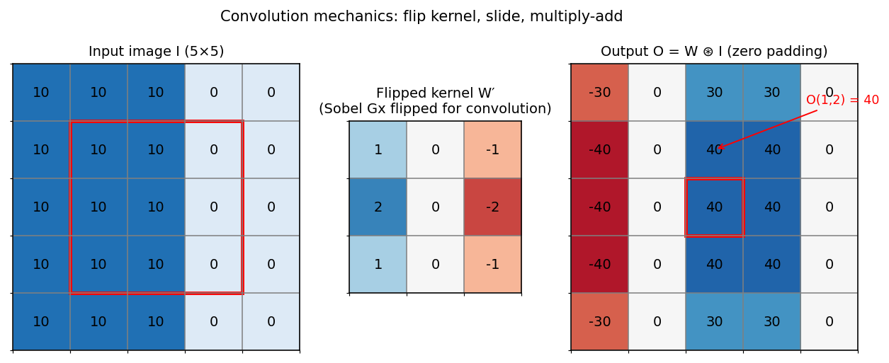
EN: Convolution mechanics on the exact 5×5 example of §4.3 — the red 3×3 patch of the input, the 180°-flipped Sobel kernel, and the highlighted output pixel O(1, 2) = 40. Note the −40/−30 left column: a pure zero-padding artifact. BN: §4.3-এর সেই 5×5 উদাহরণ — লাল ঘেরা 3×3 patch, উল্টানো Sobel kernel, আর output pixel O(1, 2) = 40। বাঁ-ধারের −40/−30 কলামটা শুধুই zero padding-এর artifact।

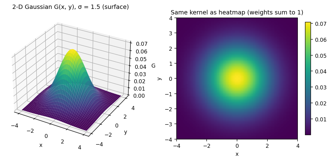
EN: The 2-D Gaussian (σ = 1.5) as a 3-D bell surface and as a heatmap. Center pixels dominate; weights decay smoothly and sum to 1. BN: 2-D Gaussian (σ = 1.5) — ঘণ্টা-আকৃতির surface আর heatmap। কেন্দ্রের weight সবচেয়ে বড়, দূরত্বের সাথে মসৃণভাবে কমে, যোগফল ১।

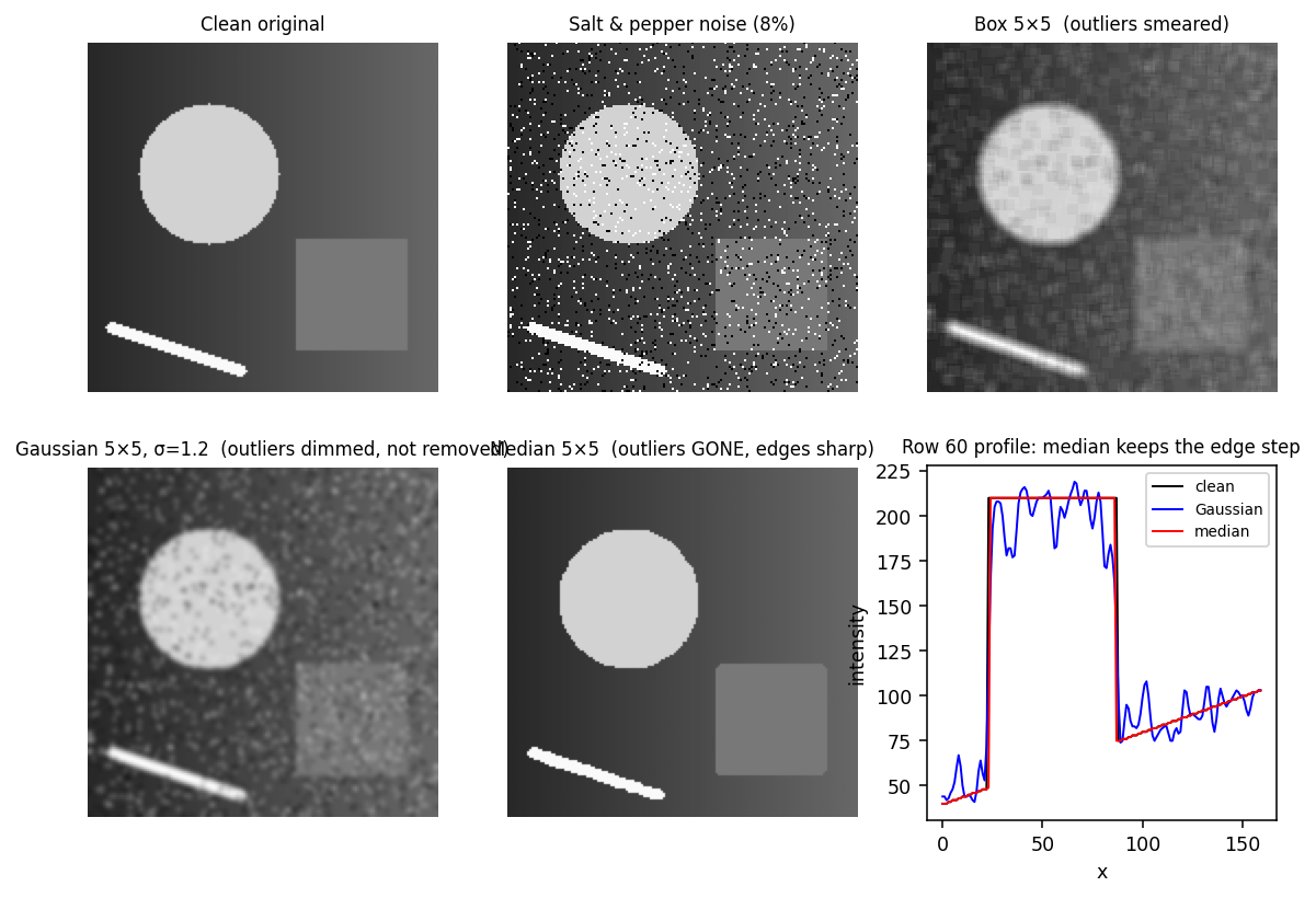
EN: Salt-and-pepper noise: box and Gaussian only dim the outliers into gray smudges; the median removes them completely while keeping edges sharp (see the row-profile plot, bottom right). BN: salt & pepper noise-এ box আর Gaussian outlier-গুলোকে শুধু ধূসর দাগে পরিণত করে; median সেগুলো পুরোপুরি মুছে দেয় আর edge-ও ধারালো রাখে (নিচে-ডানে profile plot দেখো)।

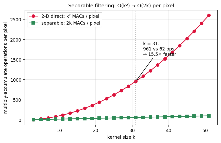
EN: Multiply-accumulate operations per pixel: k² for direct 2-D filtering vs 2k for two 1-D passes. At k = 31 that is 961 vs 62 → 15.5× faster. BN: প্রতি pixel-এ অপারেশন: সরাসরি 2-D হলে k², separable হলে মাত্র 2k। k = 31 হলে 961 বনাম 62 — সাড়ে ১৫ গুণ দ্রুত।

EN: Sobel on a synthetic shape image: Ix responds to vertical edges, Iy to horizontal ones; |∇I| combines both; θ = atan2(Iy, Ix) color-codes the gradient direction (shown only where the magnitude is significant). BN: Sobel-এর পুরো গল্প: Ix ধরে খাড়া edge, Iy ধরে আনুভূমিক edge; |∇I| দুটোকে মেলায়; θ = atan2(Iy, Ix) gradient-এর দিক রঙে দেখায় (যেখানে magnitude বড়, শুধু সেখানে)।

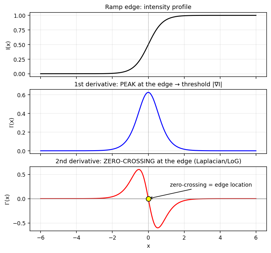
EN: A ramp edge: the 1^st derivative peaks exactly at the edge (threshold |∇I| to detect it); the 2^nd derivative crosses zero there (Laplacian/LoG zero-crossing detection). BN: ramp edge-এ 1^st derivative-এর চূড়া ঠিক edge-এর ওপরে, আর 2^nd derivative সেখানে শূন্য পেরোয় — এই zero-crossing-ই Laplacian/LoG-এর edge খোঁজার উপায়।

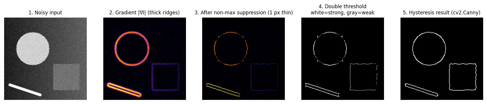
EN: The Canny pipeline on a noisy synthetic image: thick gradient ridges → 1-px-thin ridges after non-maximum suppression → strong (white) / weak (gray) after the double threshold → final connected edges after hysteresis. BN: noisy ছবিতে Canny-র ধাপগুলো: মোটা gradient ridge → NMS-এর পরে ১-pixel চিকন → double threshold-এ সাদা (strong) / ধূসর (weak) → hysteresis-এর পরে জোড়া-লাগানো চূড়ান্ত edge।

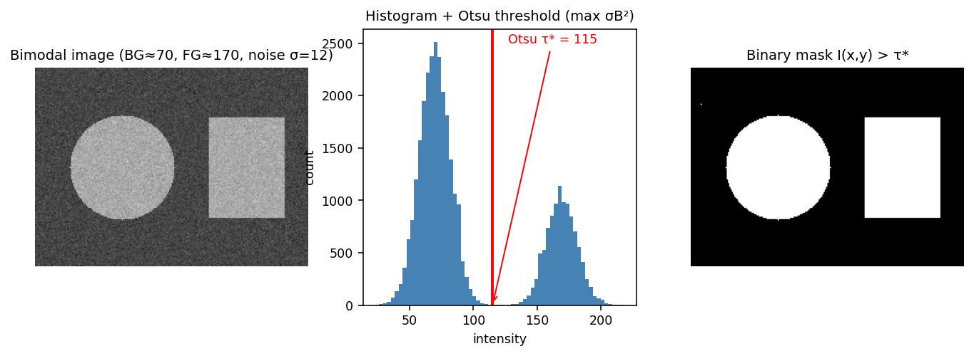
EN: A bimodal image (background ≈ 70, foreground ≈ 170, noise σ = 12): Otsu places τ in the histogram valley by maximizing σ_B², producing a clean binary mask.* BN: bimodal ছবিতে Otsu σ_B² সর্বোচ্চ করে τ-কে histogram-এর উপত্যকায় বসায় — ফলাফল পরিষ্কার binary mask।*

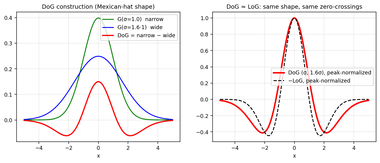
EN: Left — subtracting a wide Gaussian from a narrow one creates the Mexican-hat profile. Right — peak-normalized DoG vs −LoG: same shape, same zero-crossings, which is why DoG ≈ LoG. BN: বাঁয়ে — সরু Gaussian থেকে চওড়া Gaussian বিয়োগ করলেই Mexican hat। ডানে — normalize করলে DoG আর −LoG প্রায় একই বক্ররেখা, zero-crossing-ও এক — এজন্যই DoG ≈ LoG।

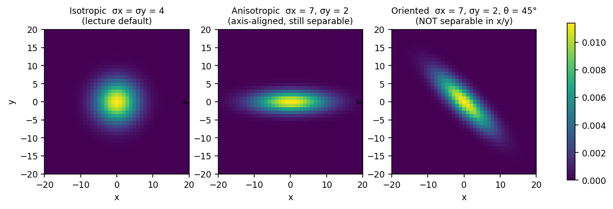
EN: Isotropic Gaussian (σx = σy, the lecture default), axis-aligned anisotropic (σx ≠ σy — still separable), and a 45°-rotated oriented Gaussian (no longer separable along x/y). Relevant for the transfer-tier questions. BN: isotropic Gaussian (σx = σy), axis-aligned anisotropic (σx ≠ σy — এখনো separable), আর ৪৫° ঘোরানো oriented Gaussian (x/y বরাবর আর separable নয়)। Mock exam-এর transfer প্রশ্নে এটাই লাগবে।

---

§6. Algorithms & Code

6.1 Hand-convolution recipe (the exam algorithm)

INPUT: image I, kernel W (k×k), border rule
1. Flip W by 180° → W′ (skip mentally if W is symmetric; flip signs if anti-symmetric).
2. For every output pixel (x, y):
   a. Extract the k×k patch of I centered at (x, y), applying the border rule for
      out-of-image samples (exam default: zero padding).
   b. Multiply patch and W′ element-wise; sum the k² products.
   c. Write the sum to O(x, y).
3. State whether the result is signed (derivative kernels!) and interpret signs.

Time per pixel: O(k²), full image O(W·H·k²); separable kernels: O(W·H·2k).

6.2 Box / Gaussian / Median (exercise sheet 3, task 1)

import cv2, numpy as np

def filter_box(img, ksize=5):
    return cv2.boxFilter(img, -1, (ksize, ksize))

def filter_gauss(img, ksize=5, sigma=1.0):
    return cv2.GaussianBlur(img, (ksize, ksize), sigma)

def filter_median(img, ksize=5):
    return cv2.medianBlur(img, ksize)

def filter_gauss_manual(img, ksize=5, sigma=1.0):
    ax = np.arange(-(ksize // 2), ksize // 2 + 1)
    xx, yy = np.meshgrid(ax, ax)
    kernel = np.exp(-(xx**2 + yy**2) / (2 * sigma**2))
    kernel /= kernel.sum()                      # weights MUST sum to 1 (Section 4.8)
    return cv2.filter2D(img.astype(np.float32), -1, kernel,
                        borderType=cv2.BORDER_REFLECT)

6.3 Manual 2-D convolution from scratch (no cv2.filter2D)

def conv2d_manual(I, K):
    Kf = K[::-1, ::-1]                          # step 1: flip 180°
    kh, kw = Kf.shape
    ph, pw = kh // 2, kw // 2
    Ip = np.pad(I.astype(float), ((ph, ph), (pw, pw)))   # zero padding
    O = np.zeros_like(I, dtype=float)
    for y in range(I.shape[0]):
        for x in range(I.shape[1]):
            O[y, x] = np.sum(Ip[y:y+kh, x:x+kw] * Kf)    # multiply-add
    return O

6.4 Separable Gaussian blur

def gauss_blur_separable(img, sigma):
    k = max(3, int(6 * sigma) | 1)              # kernel size ≈ 6σ, forced odd
    ax = np.arange(-(k // 2), k // 2 + 1)
    g = np.exp(-ax**2 / (2 * sigma**2))
    g /= g.sum()
    tmp = cv2.filter2D(img.astype(np.float32), -1, g[None, :])   # 1-D horizontal
    return cv2.filter2D(tmp, -1, g[:, None])                     # 1-D vertical

6.5 Sobel + gradient magnitude/orientation + threshold mask (sheet 3, task 4)

def filter_sobel(img):
    gx = np.array([[-1, 0, 1], [-2, 0, 2], [-1, 0, 1]], np.float32)
    gy = gx.T
    Ix = cv2.filter2D(img.astype(np.float32), -1, gx)
    Iy = cv2.filter2D(img.astype(np.float32), -1, gy)
    mag = np.sqrt(Ix**2 + Iy**2)
    theta = np.arctan2(Iy, Ix)                  # orientation in radians
    return mag, theta, Ix, Iy

def apply_threshold(img, tau):
    return (img > tau).astype(np.uint8)

def apply_mask(img, mask, color=(255, 255, 255)):
    out = img.copy(); out[mask == 1] = color; return out

6.6 Trial-exam Q2c verification (8×8 diamond ⊛ [−1, 0, 1])

import numpy as np, scipy.signal as sg
I = np.array([
 [0,0,0,0,0,0,0,0],[0,0,0,0,0,0,0,0],[0,0,1,1,1,0,0,0],
 [0,1,1,1,1,1,0,0],[0,1,1,1,1,1,0,0],[0,1,1,1,1,0,0,0],
 [0,0,1,1,0,0,0,0],[0,0,0,0,0,0,0,0]], dtype=int)
K = np.array([[-1, 0, 1]])
print(sg.convolve2d(I, K, mode='same', boundary='fill', fillvalue=0))
# matches the matrix derived by hand in Section 4.4

6.7 Image stacking to denoise (sheet 3, task 3)

N = len(imgs_dark_noise); darkening_factor = 0.1
stacked = np.zeros_like(imgs_dark_noise[0], dtype=np.float64)
for f in imgs_dark_noise:
    stacked += f.astype(np.float64)
restored = np.clip(stacked / (N * darkening_factor), 0, 255).astype(np.uint8)
# averaging N frames shrinks zero-mean noise std by 1/√N; dividing by the
# darkening factor restores brightness  →  SNR improves by √N

6.8 Otsu from scratch + Otsu vs adaptive

def otsu(gray):
    hist, _ = np.histogram(gray, bins=256, range=(0, 256))
    p = hist / gray.size
    w0 = np.cumsum(p)                            # w0(t)
    mu = np.cumsum(p * np.arange(256))           # running Σ i·p_i
    muG = mu[-1]
    sigma_b2 = (muG * w0 - mu)**2 / (w0 * (1 - w0) + 1e-12)   # = w0·w1·(mu0-mu1)²
    return np.argmax(sigma_b2)

# library versions:
_, otsu_bin = cv2.threshold(gray, 0, 255, cv2.THRESH_BINARY + cv2.THRESH_OTSU)
adaptive = cv2.adaptiveThreshold(gray, 255, cv2.ADAPTIVE_THRESH_MEAN_C,
                                 cv2.THRESH_BINARY, blockSize=25, C=10)
# On a vignetted text scan: adaptive recovers the text, Otsu fails because
# the global histogram is no longer bimodal (Section 4.21).

6.9 DoG, gradient removal, unsharp masking, Canny

def DoG(img, sigma1=1.0, sigma2=1.6):            # narrow − wide ≈ −(k−1)σ²·∇²G
    return (cv2.GaussianBlur(img, (0, 0), sigma1)
            - cv2.GaussianBlur(img, (0, 0), sigma2))

def remove_linear_gradient(img):                 # trial-exam Q2biv
    blur = cv2.GaussianBlur(img, (0, 0), sigmaX=51)
    return cv2.subtract(img, blur) + 128         # high-pass + offset

def unsharp_mask(img, sigma=2.0, lam=1.0):       # transfer-tier topic
    blur = cv2.GaussianBlur(img.astype(np.float32), (0, 0), sigma)
    return np.clip(img + lam * (img - blur), 0, 255).astype(np.uint8)

edges = cv2.Canny(gray_uint8, threshold1=100, threshold2=200)   # T_low, T_high

বাংলা: কোড-গুলোর মূল শিক্ষা: (১) Gaussian kernel বানিয়ে অবশ্যই যোগফল দিয়ে ভাগ করো, (২) convolution-এর আগে kernel flip করো (cv2.filter2D আসলে correlation করে — symmetric kernel-এ সমস্যা নেই), (৩) float32-এ কাজ করো, নইলে uint8 overflow হবে, (৪) Otsu-র σ_B² এক লাইনে vectorize করা যায়।

---

§7. Trial-Exam Mapping

Trial-exam question	What it asks	Where in this chapter
2a	Match images ↔ Fourier power spectra	§2.3 (rules: stripes ⇒ perpendicular bright spots; noise ⇒ bright everywhere; smooth gradient ⇒ energy near center)
2bi	Purpose of the Gaussian filter	§4.8 (smoothing/noise removal without ringing — Gaussian stays Gaussian in Fourier space)
2bii	Purpose of DoG, what it approximates	§4.16 (≈ LoG; band-pass; separable ⇒ fast; SIFT scale space)
2biii	Global vs local thresholding	§4.21 (exam-ready answer included)
2biv	Remove linear brightness gradient from concrete wall	§4.22 (subtract heavy Gaussian blur = high-pass)
2c	Convolve 8×8 image with [−1, 0, 1]	§4.4 (full worked matrix) + §6.6 (code check)
2d	Filter category + more filters of that category	§4.4 interpretation (horizontal gradient/edge detector; Sobel, Prewitt, Roberts, Scharr, Laplacian, LoG, DoG, Gabor, Canny)

Detailed model answers: CVML_Trial_Exam_Analysis.md.

বাংলা: trial exam-এর প্রতিটি প্রশ্নের উত্তর এই chapter-এই আছে — টেবিলের ডান কলামের section-গুলো ধরে ধরে revise করো। বিশেষ করে 2c-র মতো হাতে-কলমে convolution আর 2bii-র DoG-উত্তরটা মুখস্থ রাখো।

---

§8. Mock Exam — 20 Questions (4 Tiers × 5)

Work through the questions first; full worked solutions follow in §8.5.

Tier A — Basic (definitions & one-liners)

A1. Define correlation and convolution of an image with a kernel. What is the single operational difference, and for which class of kernels do the two give identical results?

A2. State the purpose of the Gaussian filter and give two reasons why it is preferred over the box filter for smoothing.

A3. What does the median filter compute, why is it called non-linear, and for which noise type is it the method of choice?

A4. What is the Difference of Gaussians (DoG), what does it approximate, and name one famous algorithm that uses it.

A5. Explain the difference between global and local (adaptive) thresholding in 2–3 sentences. When is the local variant indispensable?

Tier B — Intuitive (why-questions)

B1. Why must the weights of any smoothing kernel sum to exactly 1? Predict what happens to a constant image of value 100 if the weights sum to 1.2.

B2. Using the Fourier domain, explain why the box filter produces ringing artifacts while the Gaussian filter does not.

B3. "An edge in an image is just the gradient." Refute this with two counterexamples from the lecture, and state the correct relation between edges, the 1^st derivative, and the 2^nd derivative.

B4. Why must an image be low-pass filtered before subsampling when building an image pyramid? Which theorem is at work and what artifact appears otherwise?

B5. The Sobel x-kernel weights the middle row by 2 while Prewitt uses all ones. Explain what both operators are really doing (decomposition!), and why Sobel's weighting is the better choice.

Tier C — Harder (multi-step computation)

C1. Convolve (true convolution, not correlation!) the 5×5 image below with the Sobel y-kernel. Give the full valid (3×3) output and explain the sign of your result. Then state the valid output for plain correlation.

\[ \begin{aligned} I = 0 0 0 0 0 Sy = -1 -2 -1 \\ 0 0 0 0 0 0 0 0 \\ 10 10 10 10 10 1 2 1 \\ 10 10 10 10 10 \\ 10 10 10 10 10 \end{aligned} \]

C2. A 10-pixel image has the 4-bin histogram h = [4, 2, 1, 3] for intensity levels {0, 1, 2, 3}. Compute Otsu's threshold: evaluate σ_B²(t) = w₀w₁(μ₀ − μ₁)² for every candidate t ∈ {0, 1, 2} and state the optimal split.

C3. Apply the Sobel masks Sx = [−1 0 1; −2 0 2; −1 0 1] and Sy = Sxᵀ as correlation (as in the lecture) to the center of the patch below. Compute Ix, Iy, the gradient magnitude, and the orientation θ = atan2(Iy, Ix).

\[ \begin{aligned} P = 0 0 10 \\ 0 10 10 \\ 10 10 10 \end{aligned} \]

C4. A 3×3 window reads [12, 10, 11; 250, 11, 9; 10, 12, 0] (one salt pixel 250, one pepper pixel 0). Compute the output of (a) a 3×3 box filter, (b) a 3×3 median filter, at the center. Which is closer to the plausible true value ≈ 11, and why?

C5. You blur a Full-HD frame (1920 × 1080) with a k = 31 Gaussian. Compute the number of multiply-accumulate operations per pixel and for the whole frame for (a) direct 2-D convolution and (b) separable filtering, and the resulting speed-up factor.

Tier D — Transfer (slightly beyond the lecture)

D1. The lecture used isotropic Gaussians (one σ). Write down the anisotropic, oriented 2-D Gaussian with σx ≠ σy and orientation angle α. Name one use case, and discuss: is it still separable?

D2. Write the bilateral filter equation and explain, term by term, why it smooths noise yet preserves edges, while a Gaussian of the same spatial σ blurs them. Why can it not be implemented as a convolution?

D3. Derive unsharp masking as a single linear filter: show that I + λ(I − G ⊛ I) equals one kernel applied to I, compute that effective 1-D kernel for g = [0.25, 0.5, 0.25] and λ = 1, and discuss one risk of large λ.

D4. The Scharr operator uses the smoothing vector [3, 10, 3]/16 instead of Sobel's [1, 2, 1]/4. What deficiency of Sobel does it address, in which situations does the difference matter, and what stays exactly the same?

D5. A document photo has a strong vignette (bright center, dark corners). Global Otsu produces garbage. Explain precisely why Otsu fails here (histogram argument), then design a two-stage pipeline that fixes it using only techniques from this chapter, and name the lecture's three remedies for failing Otsu.

---

§8.5 Solutions

Tier A solutions

A1. Correlation: \((W \odot I)(x,y) = \Sigma _{i} \Sigma _{j} W(i,j)\cdot I(x+i, y+j)\) — slide the kernel as written, multiply, sum. Convolution: \((W \circledast I)(x,y) = \Sigma _{i} \Sigma _{j} W(i,j)\cdot I(x-i, y-j)\) — identical procedure after rotating the kernel by 180° (mirror both axes). That flip is the only operational difference, and it buys associativity + commutativity (filter chains can be pre-combined) and the convolution theorem. For symmetric kernels (box, Gaussian, Laplacian) flip changes nothing → both operations coincide; for anti-symmetric kernels (Sobel, [−1, 0, 1]) the sign of the output flips. বাংলা: পার্থক্য একটাই — convolution আগে kernel ১৮০° উল্টে নেয়; symmetric kernel-এ দুটো সমান, anti-symmetric-এ চিহ্ন উল্টে যায়।

A2. Purpose: smoothing / noise suppression — a weighted average where near pixels count more, weights from the Gaussian bell curve. Better than box because (1) its Fourier transform is again a Gaussian: smooth roll-off of high frequencies with no oscillating side lobes ⇒ no ringing, no frequency is amplified or inverted; (2) the smooth, rotationally symmetric weighting treats all directions equally and gives near pixels appropriately more influence, while still being separable and therefore fast. বাংলা: Gaussian = ringing-ছাড়া smoothing; কারণ Fourier domain-এও সে Gaussian — ধারালো কাটা নেই, আর separable বলে দ্রুত।

A3. It replaces each pixel by the median of its neighbourhood window. Non-linear because median(a + b) ≠ median(a) + median(b) (counterexample in §4.10) — so no kernel/convolution can express it. It is the method of choice for salt-and-pepper (impulse) noise: extreme outliers never enter the output as long as they are a minority of the window, and step edges are preserved instead of blurred. বাংলা: median outlier-কে স্রেফ উপেক্ষা করে — তাই salt & pepper-এ অপ্রতিদ্বন্দ্বী; আর এটা linear নয় বলে কোনো kernel দিয়ে লেখা যায় না।

A4. \(DoG = G_\sigma _{1} - G_\sigma _{2}\) (two Gaussians of different width, subtracted). It approximates the Laplacian of Gaussian (LoG) — \(DoG \approx (k-1)\sigma ^{2}\cdot \nabla ^{2}G\) — i.e. a band-pass / blob detector, but much cheaper because Gaussians are separable and the blurred images are reused. Famous user: SIFT, which builds its scale space from DoG levels and additionally reads off the scale σ at which a structure responds most. বাংলা: DoG = দুই Gaussian-এর বিয়োগ ≈ LoG; সস্তা কারণ separable; SIFT-এর scale space-এর ভিত্তি।

A5. Global: one threshold τ for the whole image — works only if the histogram is bimodal with a clean valley, i.e. uniform lighting. Local/adaptive: a per-pixel τ(x, y) computed from a window around the pixel (local mean, possibly std: e.g. τ = μ_xy − C). Indispensable when illumination varies across the image — vignetting, brightness gradients, shadowed document scans — because then no single global value separates foreground from background everywhere. বাংলা: global = গোটা ছবিতে এক τ; local = প্রতি pixel-এ পাড়া-প্রতিবেশী দেখে আলাদা τ; আলো অসমান হলে local ছাড়া গতি নেই।

Tier B solutions

B1. Feeding a constant image c through a linear filter gives \(O = c \cdot \Sigma W\) (§4.8). To leave flat regions — and overall brightness — unchanged we need ΣW = 1. With ΣW = 1.2 the constant-100 image becomes constant 120: a 20% global brightening, and any further filter pass brightens again. (Contrast: derivative kernels deliberately sum to 0 so flat regions output 0.) বাংলা: যোগফল ১ না হলে সমতল অঞ্চলের উজ্জ্বলতাই বদলে যায় — ১.২ হলে ১০০ হয়ে যায় ১২০; derivative kernel-এর যোগফল আবার ইচ্ছা করেই ০।

B2. Convolution in image space = multiplication in Fourier space. The box's Fourier transform is a sinc — decaying oscillations that dip below zero. Multiplying the image spectrum by it leaves alternating attenuated/negated frequency bands ⇒ visible ripples (ringing) next to edges. The Gaussian's transform is a positive, monotonically decaying Gaussian: smooth roll-off, no side lobes, no sign flips ⇒ no ringing. (The sinc filter is the extreme case: hard cut-off in frequency = sinc in space = maximal ringing.) বাংলা: box-এর Fourier রূপ দুলতে-থাকা sinc (ঋণাত্মকও হয়) → ঢেউ; Gaussian-এর Fourier রূপ মসৃণ ধনাত্মক Gaussian → কোনো ঢেউ নেই।

B3. Lecture counterexamples: (1) a noisy flat region has constantly high gradient yet contains no edge; (2) a smooth/blurred object contour is a strong perceptual edge although the per-pixel gradient is small (and a perfectly flat region has neither). Correct relation: an ideal edge is a localized, coherent intensity transition — it shows up as a peak of the 1^st derivative and a zero-crossing of the 2^nd derivative; gradient magnitude alone, without localization/coherence (NMS, hysteresis!), is not yet an edge. বাংলা: gradient বড় মানেই edge নয় (noise!), gradient ছোট মানেই edge নেই তা-ও নয় (আবছা boundary)। edge = 1^st derivative-এর peak = 2^nd derivative-এর zero-crossing।

B4. Subsampling by 2 halves the sampling rate; by Nyquist, the new grid can only represent frequencies up to half of what the old one could. Any finer detail still present aliases: it reappears as false coarse patterns (Moiré, jagged stair-stepping) that no later processing can undo. Gaussian-blurring first removes those unrepresentable high frequencies, so each pyramid level is a faithful coarse version — "smooth, then take every second pixel of every second row." বাংলা: আগে blur না করলে Nyquist-সীমার ওপরের frequency গুলো ভুয়া প্যাটার্ন (aliasing) হয়ে ফিরে আসে; Gaussian আগে সেগুলো মুছে দেয় বলেই pyramid-এর প্রতিটি ধাপ বিশ্বস্ত থাকে।

B5. Both are the outer product (derivative) ⊗ (perpendicular smoothing): Prewitt = [−1 0 1] ⊗ [1 1 1]/3 (box smoothing), Sobel = [−1 0 1] ⊗ [1 2 1]/4 (binomial ≈ Gaussian smoothing). The smoothing perpendicular to the derivative suppresses noise before differencing — legal to pre-combine thanks to associativity: D ⊛ (L ⊛ I) = (D ⊛ L) ⊛ I. Sobel's [1 2 1] is better because the Gaussian-like weighting (i) suppresses noise with weights matched to distance, (ii) is closer to rotationally symmetric, giving more accurate, less direction-biased gradients than the box. বাংলা: দুটোই = derivative ⊗ smoothing; Sobel-এর [1 2 1] হলো ছোট্ট Gaussian — box-এর চেয়ে ভালো noise দমন আর কম দিক-পক্ষপাত।

Tier C solutions

C1. Flip Sy by 180° → \([1 2 1; 0 0 0; -1 -2 -1]\). Each valid output = (weighted row above) − (weighted row below), weights (1, 2, 1), i.e. O = 4·I(row above) − 4·I(row below) for constant rows. Valid rows use image rows (0,1,2), (1,2,3), (2,3,4):

row (0,1,2): above = 0·4 = 0,  below = 10·4 = 40  →  0 − 40 = −40
row (1,2,3): above = 0,        below = 40         →  −40
row (2,3,4): above = 40,       below = 40         →  0

O_valid (convolution) =  −40 −40 −40        O_valid (correlation) =  40 40 40
                         −40 −40 −40                                 40 40 40
                           0   0   0                                  0  0  0

Sign: the flipped kernel computes (top − bottom); intensity increases downward across the edge, so top − bottom < 0 ⇒ −40. Correlation computes (bottom − top) ⇒ +40. (Both verified numerically.) বাংলা: convolution-এ kernel উল্টে যায় বলে উত্তর −৪০, correlation-এ +৪০ — মান এক, চিহ্ন বিপরীত; এটাই anti-symmetric kernel-এর ফাঁদ।

C2. N = 10, p = [0.4, 0.2, 0.1, 0.3]; Σ i·p_i = 0 + 0.2 + 0.2 + 0.9 = 1.3 = μ_G.

t = 0: w₀ = 0.4, μ₀ = 0;        w₁ = 0.6, μ₁ = (0.2+0.2+0.9)/0.6 = 13/6 ≈ 2.1667
       σ_B² = 0.4·0.6·(2.1667)² = 0.24·4.6944 ≈ 1.127
t = 1: w₀ = 0.6, μ₀ = 0.2/0.6 = 0.3333;  w₁ = 0.4, μ₁ = (0.2+0.9)/0.4 = 2.75
       σ_B² = 0.6·0.4·(2.75 − 0.3333)² = 0.24·(2.4167)² = 0.24·5.8403 ≈ 1.402   ← MAX
t = 2: w₀ = 0.7, μ₀ = 0.4/0.7 = 0.5714;  w₁ = 0.3, μ₁ = 0.9/0.3 = 3.0
       σ_B² = 0.7·0.3·(3.0 − 0.5714)² = 0.21·5.898 ≈ 1.239

Optimal threshold t* = 1: class C₀ = {0, 1} (6 pixels), class C₁ = {2, 3} (4 pixels), σ_B² ≈ 1.402. বাংলা: তিনটা t-এর σ_B² বের করে সবচেয়ে বড়টা নাও — এখানে t = 1; পরীক্ষায় ঠিক এই টেবিল-পদ্ধতিই দেখাবে।

C3. Correlation = multiply position-wise as written, then sum.

Ix = (−1)·0 + 0·0 + 1·10  +  (−2)·0 + 0·10 + 2·10  +  (−1)·10 + 0·10 + 1·10
   = 10 + 20 + (−10 + 10) = 30
Iy = (−1)·0 + (−2)·0 + (−1)·10  +  0 + 0 + 0  +  1·10 + 2·10 + 1·10
   = −10 + 40 = 30
|∇I| = √(30² + 30²) = 30√2 ≈ 42.43
θ = atan2(30, 30) = 45°

The gradient points at 45° (down-right in image coordinates, toward brighter pixels); the edge itself runs perpendicular, at 135° — consistent with the anti-diagonal edge in the patch. বাংলা: Ix = Iy = 30, তাই magnitude 30√2 ≈ 42.4 আর θ = 45° — কোণাকুণি edge-এ ঠিক যেমনটা আশা করা যায়।

C4. (a) Box: sum = 12+10+11+250+11+9+10+12+0 = 325, output = 325/9 ≈ 36.1. (b) Median: sorted = [0, 9, 10, 10, 11, 11, 12, 12, 250] → 5^th value = 11. The median (11) hits the plausible true value exactly: it discards both impulse outliers because rank statistics ignore how extreme values are, only where they rank. The box filter lets the 250 (and the 0) leak arithmetically into the average, dragging it to 36 — more than 3× the true value. বাংলা: গড় outlier-এর টানে ৩৬-এ চলে যায়, median নির্বিকারভাবে ১১ — salt & pepper-এ median-এর জয় এখানেই।

C5. Pixels: 1920 · 1080 = 2,073,600.

(a) direct 2-D: 31² = 961 MACs/pixel → 2,073,600 · 961 ≈ 1.99 × 10⁹ MACs/frame
(b) separable:  2·31 = 62 MACs/pixel → 2,073,600 · 62  ≈ 1.29 × 10⁸ MACs/frame
speed-up: 961 / 62 = 15.5×

At 30 fps that is ~60 GMAC/s vs ~3.9 GMAC/s — separability decides whether real-time is feasible. বাংলা: প্রতি pixel-এ ৯৬১ বনাম ৬২ অপারেশন — separability মানে সাড়ে ১৫ গুণ গতি, real-time-এর চাবিকাঠি।

Tier D solutions

D1. Rotate coordinates by α and give each axis its own σ:

\[ \begin{aligned} x' = x\cdot \cos \alpha + y\cdot \sin \alpha y' = -x\cdot \sin \alpha + y\cdot \cos \alpha \\ G(x, y) = (1 / (2\pi \sigma x \sigma y)) \cdot \exp ( -( x'^{2}/(2\sigma x^{2}) + y'^{2}/(2\sigma y^{2}) ) ) \end{aligned} \]

Isotropic = special case σx = σy (any α). Use cases: smoothing along an edge/line direction without blurring across it; modeling directional motion blur; the elongated envelope of Gabor filters. Separability: for α = 0 (axis-aligned) yes — G = g_σx(x)·g_σy(y), two 1-D passes with different σ. For a rotated kernel (α ≠ 0, σx ≠ σy) it is not separable along the image's x/y axes (the exponent contains a cross term xy); it is separable along the rotated axes x′, y′, which is impractical on a pixel grid — so implementations either filter along resampled lines or apply the full 2-D kernel. বাংলা: σx ≠ σy দিলে Gaussian ডিম্বাকৃতি হয়, α দিয়ে ঘোরানো যায়; axis-aligned হলে এখনো separable, কিন্তু ঘোরানো হলে x/y বরাবর আর separable নয় (exponent-এ xy term ঢুকে যায়)।

D2.

BF[I](p) = (1/W_p) Σ_q  G_σs(‖p − q‖) · G_σr(|I(p) − I(q)|) · I(q)
W_p      =          Σ_q  G_σs(‖p − q‖) · G_σr(|I(p) − I(q)|)

Two kernels multiply: the spatial kernel G_σs (near pixels count more — same as Gaussian) and the range kernel G_σr (pixels with similar intensity count more). At an edge, pixels on the far side differ strongly in intensity → their range weight ≈ 0 → they are excluded from the average → the edge stays sharp, while same-side pixels still average their noise away. A plain Gaussian has no range term and mixes across the edge. It cannot be a convolution because the weights depend on the image content at each position (via I(p) − I(q)): the kernel changes per pixel, so the operation is shift-variant and non-linear; W_p must renormalize the weights at every pixel. বাংলা: bilateral = কাছের এবং একই-রকম-উজ্জ্বল pixel-দেরই গড়; edge-এর ওপারের pixel intensity-তে আলাদা বলে weight শূন্য — তাই edge বাঁচে। weight ছবির ওপর নির্ভর করে বলে এটা আর convolution নয়।

D3.

sharpened = I + λ(I − G ⊛ I) = (1 + λ)·(δ ⊛ I) − λ·(G ⊛ I) = [(1 + λ)δ − λG] ⊛ I

(δ = identity kernel: 1 at center.) One linear kernel — a "high-boost" filter. For g = [0.25, 0.5, 0.25], λ = 1:

k = 2·[0, 1, 0] − [0.25, 0.5, 0.25] = [−0.25, 1.5, −0.25]
check: −0.25 + 1.5 − 0.25 = 1 ✓ (brightness preserved)  — center boosted, neighbours negative

Risks of large λ: noise lives in the high frequencies, so it is amplified together with real detail, and overshoot/halo artifacts appear at strong edges (values pushed past the original range, visible bright/dark rims). Connection: (I − G ⊛ I) is exactly a high-pass — for the masking step, DoG with a tiny inner σ. বাংলা: unsharp masking = মূল ছবি + λ·(high-frequency অংশ), এক kernel-এ লেখা যায়: (1+λ)δ − λG। λ বেশি হলে noise-ও ধারালো হয় আর edge-এর পাশে halo পড়ে।

D4. Sobel's [1, 2, 1] smoothing is only a crude Gaussian: its gradient direction estimates are biased for edges that are neither axis-aligned nor exactly diagonal (poor rotational symmetry). Scharr's [3, 10, 3]/16 weighting is numerically optimized so the operator's frequency response is as direction-independent as possible → markedly more accurate gradient orientations. It matters wherever angles feed downstream computations: Canny's NMS direction bins, structure tensors, optical flow, orientation histograms (SIFT/HOG). What stays the same: the construction (derivative [−1, 0, 1] ⊗ smoothing), size 3×3, separability, cost, and the derivative row summing to 0 / smoothing summing to 1. বাংলা: Sobel-এর কোণ-নির্ণয় তির্যক edge-এ একটু বাঁকা হয়; Scharr-এর [3, 10, 3] ওজন rotational symmetry ভালো করে — দিক যত গুরুত্বপূর্ণ (NMS, optical flow), Scharr তত দরকারি; গঠন আর খরচ Sobel-এর মতোই।

D5. Why Otsu fails: Otsu sees only the global histogram. The vignette multiplies/shifts intensities position-dependently, so "paper" pixels range from bright (center) to dark (corners) and overlap the "ink" range; the histogram's two modes smear into one broad lump with no valley — no single τ separates the classes anywhere, and σ_B²(t) has no meaningful maximum. Pipeline fix: (1) Illumination flattening: estimate the vignette with a very large-σ Gaussian blur and subtract it (or divide, since vignetting is multiplicative) — §4.22 — restoring a bimodal histogram; (2) Threshold: now apply Otsu globally, or skip step 1 and use adaptive thresholding τ(x, y) = μ_xy − C with a window larger than a letter but smaller than the vignette scale. Lecture's three Otsu remedies: low-pass filter the image first; compute the histogram only from pixels near edges (e.g. high |Laplacian|); subdivide the image into blocks and run Otsu per block. বাংলা: vignette histogram-এর দুই চূড়া গলিয়ে এক করে দেয়, তাই global Otsu অন্ধ। সমাধান: আগে বড়-σ Gaussian দিয়ে আলো আন্দাজ করে বাদ দাও, তারপর Otsu — অথবা সরাসরি adaptive thresholding; আর lecture-এর তিন দাওয়াই: আগে blur, শুধু edge-ঘেঁষা pixel-এর histogram, block-ভাগ করে Otsu।

---

§9. Exam-Day Cheat Sheet

Core formulas (memorize cold):

correlation:  (W ⊙ I)(x,y) = Σ W(i,j)·I(x+i, y+j)        convolution: flip W 180° first
Gaussian:     G(x,y) = (1/(2πσ²))·e^(−(x²+y²)/(2σ²))     1-D: g(x) = (1/(√(2π)σ))·e^(−x²/(2σ²))
separability: G(x,y) = g(x)·g(y)   ⇒   O(k²) → O(2k) per pixel,  speed-up k/2
derivatives:  forward [−1, 1] (O(h));  central ½[−1, 0, 1] (O(h²));  second [1, −2, 1]
Sobel:        Sx = [−1 0 1] ⊗ [1 2 1]/4;   Prewitt uses [1 1 1]/3;   Scharr uses [3 10 3]/16
gradient:     |∇I| = √(Ix² + Iy²),   θ = atan2(Iy, Ix),   edge ⊥ θ
Laplacian:    N4 [0 1 0; 1 −4 1; 0 1 0]    N8 [1 1 1; 1 −8 1; 1 1 1]    (sum = 0)
LoG:          ∇²G = ((x² + y² − 2σ²)/σ⁴)·G        kernel zero at r = σ√2
DoG:          G_σ₁ − G_σ₂ ≈ (k−1)σ²·∇²G           (heat eq.: ∂G/∂σ = σ∇²G);  SIFT k = 1.6
Canny:        Gauss → Sobel → NMS → double threshold → hysteresis
Otsu:         σ_B²(t) = w₀w₁(μ₀ − μ₁)²  → maximize over t      (σ_G² = σ_W² + σ_B²)
adaptive:     τ(x, y) = μ_xy − C   (per-pixel, from local window)
unsharp:      I + λ(I − G ⊛ I) = [(1+λ)δ − λG] ⊛ I

Decision table:

Situation	Reach for
Gaussian sensor noise	Gaussian filter
Salt & pepper noise	Median filter
Edge strength + direction	Sobel → magnitude + atan2
Clean 1-px connected edges	Canny
Blob / scale detection	DoG (≈ LoG)
Bimodal histogram, even light	Otsu
Uneven illumination	Adaptive threshold (or blur-subtract first)
Need speed with big kernels	Separable filtering

Sanity checks before submitting an answer: smoothing kernel sums to 1; derivative kernel sums to 0; convolution = correlation only for symmetric kernels; signed outputs need interpretation (which side is bright?); zero padding fakes edges at the border; output shrinks by k−1 without padding.

English mantras: 1. "Convolution flips, correlation doesn't — symmetric kernels can't tell." 2. "Gaussian in, Gaussian out (Fourier) — that's why no ringing." 3. "Smooth sums to one, derivative sums to zero." 4. "Edge = first-derivative peak = second-derivative zero-crossing." 5. "DoG approximates LoG: subtract two blurs, get a band-pass — SIFT's engine." 6. "Otsu maximizes w₀w₁(μ₀−μ₁)²; uneven light? Go adaptive." 7. "Canny: smooth, differentiate, thin, double-threshold, connect."

বাংলা মন্ত্র: 1. বাংলা: convolution মানেই আগে kernel উল্টাও — Sobel-এ ভুললে চিহ্ন উল্টে যাবে। 2. বাংলা: smoothing kernel-এর যোগফল ১, derivative kernel-এর যোগফল ০ — এই দুটো check সবার আগে। 3. বাংলা: Gaussian দুই জগতেই Gaussian, তাই ringing নেই — smoothing-এর প্রশ্নের default উত্তর। 4. বাংলা: edge খুঁজতে: 1^st derivative-এর চূড়া, 2^nd derivative-এর zero-crossing। 5. বাংলা: salt & pepper দেখলেই median — গড় নয়, মাঝের মান। 6. বাংলা: Otsu-র সূত্র w₀w₁(μ₀−μ₁)² — টেবিল বানাও, সবচেয়ে বড়টা নাও; আলো অসমান হলে adaptive। 7. বাংলা: Canny-র পাঁচ ধাপ: blur → gradient → চিকন করো (NMS) → দুই threshold → জোড়া লাগাও (hysteresis)।

Last-second mantra: "Flip, slide, multiply, add. Gaussian = smooth without ringing. Median kills salt & pepper. Sobel = derivative ⊗ smoothing. DoG ≈ LoG. Otsu maximizes between-class variance. Uneven light → adaptive."