Chapter 05 — Features: Harris Corners, SIFT & Matching¶
Trial-exam weight: 10 / 110 points. The trial exam contains a numerical perspective-projection question (Q4a), a ZMNCC-failure question (Q4b) and five True/False statements about Harris and SIFT (Q4c). This chapter also feeds Chapters 6 (optical flow), 7 (transformations), 8 (epipolar geometry) and 10 (calibration) — almost every later topic starts with "first, find feature correspondences".
1. Roadmap¶
This chapter answers four questions, in order:
- What is a feature and why do we need it? A feature is a small, re-identifiable landmark in an image. All correspondence-based vision (tracking, 3-D reconstruction, panorama stitching, SLAM, AR) is built on finding the same physical point in different images.
- How do we detect good features? We formalise "a window that changes in every direction" using the SSD error surface
E(u, v), Taylor-expand it into a quadratic form with the structure tensor M, and read off flat / edge / corner from the eigenvalues of M. The Harris response \(R = \det (M) - k\cdot \operatorname{trace}(M)^{2}\) is the fast practical test; Shi–Tomasi uses \(\min (\lambda _{1}, \lambda _{2})\) instead. - How do we describe features so they survive transformations? We need scale invariance (Gaussian scale space, DoG as a cheap LoG) and rotation invariance (dominant gradient orientation). SIFT combines everything into a 128-dimensional descriptor.
- How do we match features between images? L2 distance + nearest neighbour + Lowe's ratio test (lecture threshold 0.6, paper threshold 0.8).
The mental pipeline you must be able to reproduce in the exam:
image ──► gradients (Iₓ, I_y) ──► structure tensor M ──► eigenvalues λ₁, λ₂
      ──► Harris R = det − k·trace²  ──► threshold + non-max suppression ──► keypoints
keypoints ──► scale (DoG extrema) ──► orientation (36-bin histogram)
          ──► descriptor (4×4 cells × 8 bins = 128-D) ──► L2 matching + ratio test
বাংলা: এই chapter-এ আমরা চারটা প্রশ্নের উত্তর শিখব। প্রথমত, feature কী এবং কেন দরকার — feature হলো ছবির এমন ছোট একটা চেনা-যায় এমন জায়গা, যেটা অন্য ছবিতেও খুঁজে পাওয়া যায়; tracking, 3-D reconstruction, panorama — সব কিছুর ভিত্তি এটাই। দ্বিতীয়ত, ভালো feature কীভাবে খুঁজব — window সরালে ছবি কতটা বদলায় সেটা SSD error E(u, v) দিয়ে মাপি, Taylor expansion করে structure tensor M পাই, আর M-এর eigenvalue দেখে বুঝি জায়গাটা flat, edge না corner। Harris score \(R = \det (M) - k\cdot \operatorname{trace}(M)^{2}\) হলো দ্রুত হিসাবের কৌশল। তৃতীয়ত, feature-কে এমনভাবে describe করব যাতে ছবি ঘোরালে, zoom করলে বা আলো বদলালেও সেটা একই থাকে — এর জন্য scale space, DoG আর SIFT-এর 128-dimensional descriptor। চতুর্থত, দুই ছবির feature মেলাব L2 distance আর ratio test দিয়ে। উপরের pipeline-টা পরীক্ষায় মুখস্থ লিখতে পারা চাই।
2. Concepts from Zero¶
2.1 What is a feature?¶
A feature (also: keypoint, interest point) is a small, distinctive image location together with a numerical description of its neighbourhood. Two requirements from the lecture:
- Well distinguishable — it should look different from all other locations in the image (unique).
- Well locatable — the same physical point should be findable in other images of the same scene (repeatable).
Three separate sub-tasks, and you must keep them apart in the exam:
| Task | Question it answers | Example |
|---|---|---|
| Detection | Where are good features? | Harris, Shi–Tomasi, DoG extrema, FAST |
| Description | How do we encode the neighbourhood as numbers? | SIFT 128-D vector, SURF, ORB/BRIEF |
| Matching | Which feature in image 2 corresponds to this one in image 1? | L2 nearest neighbour + ratio test |
বাংলা: Feature মানে ছবির একটা ছোট, স্বতন্ত্র জায়গা — যেমন জানালার কোণা — সাথে তার চারপাশের একটা সংখ্যাগত বর্ণনা। দুটো শর্ত: (১) distinguishable — ছবির অন্য সব জায়গা থেকে আলাদা দেখাতে হবে, (২) locatable — একই দৃশ্যের অন্য ছবিতেও সেই একই জায়গা খুঁজে পেতে হবে। কাজটা তিন ভাগে ভাগ: detection (কোথায় feature আছে), description (feature-টাকে সংখ্যা দিয়ে কীভাবে লিখব), matching (দুই ছবির feature কীভাবে মেলাব)। পরীক্ষায় এই তিনটা গুলিয়ে ফেলা চলবে না।
2.2 Why do we need correspondences at all?¶
Given a pixel \(p_{1}\) in image \(I_{1}\), we want the pixel \(p_{2}\) in image \(I_{2}\) that shows the same scene point P. We cannot compute P directly (we do not know the 3-D world), so we match image content instead. Dense matching (every pixel) is hard → we start with sparse matching: a few robust features. Applications listed in the lecture: object tracking and recognition, camera calibration, 3-D reconstruction, robot navigation, stereo disparity, motion-based segmentation, augmented reality, special effects / camera tracking in movies, image morphing, image retrieval.
বাংলা: এক ছবির pixel \(p_{1}\)-এর জন্য অন্য ছবিতে একই বাস্তব বিন্দু P-এর ছবি \(p_{2}\) খুঁজে বের করাই হলো correspondence। যেহেতু আমরা P-এর 3-D অবস্থান জানি না, তাই ছবির content মিলিয়েই কাজ চালাই। সব pixel মেলানো (dense) কঠিন, তাই অল্প কিছু শক্তিশালী feature (sparse) দিয়ে শুরু করি। ব্যবহার: tracking, recognition, calibration, 3-D reconstruction, robot navigation, AR, সিনেমার special effects ইত্যাদি।
2.3 Why corners? The matching-ambiguity argument¶
Slide a small window over the image and ask: if I shift the window slightly, does the content change?
- Flat region — shift in any direction → content barely changes → the window matches everywhere in the region → useless for matching.
- Edge — shift across the edge → big change; shift along the edge → no change → the window matches every position along the edge → still ambiguous (this is the 1-D ambiguity that reappears in Chapter 6 as the aperture problem).
- Corner — shift in any direction → big change → the window matches exactly one position → unique, ideal feature.
Analogy: a magnifying glass over a clear sky shows the same blue everywhere; over a wall edge it shows the same edge as you slide along it; over a window corner every slide shows something new — only the corner pins you to one spot.
The lecture adds a subtle point: even a patch in a homogeneous region can be a good feature if its support region is large enough that the distances to surrounding structures make it unique (the rice-plate example).
বাংলা: ছোট একটা window ছবির ওপর সামান্য সরিয়ে দেখো content বদলায় কি না। Flat জায়গায় কোনো দিকেই বদলায় না — তাই window-টা ওই region-এর সব জায়গায় match করে, কোনো কাজে আসে না। Edge-এ edge-এর আড়াআড়ি সরালে বদলায়, কিন্তু edge বরাবর সরালে বদলায় না — তাই edge-এর যেকোনো জায়গায় match করে, এটাও ambiguous (এই 1-D ambiguity-ই Chapter 6-এ aperture problem নামে ফিরে আসবে)। Corner-এ যেদিকেই সরাও content বদলায় — তাই corner ঠিক একটা জায়গাতেই match করে। এজন্যই corner সবচেয়ে ভালো feature। আরেকটা সূক্ষ্ম কথা: support region যথেষ্ট বড় হলে homogeneous জায়গার মাঝের একটা বিন্দুও ভালো feature হতে পারে, কারণ আশেপাশের কাঠামো থেকে তার দূরত্বগুলোই তাকে unique করে।
2.4 From pixels to patches: template matching, NCC, ZMNCC¶
Comparing single pixels by colour distance fails: an image has few distinct colours, so thousands of pixels look alike. Comparing whole patches (write the patch as one long vector) is far more distinctive. Three patch-similarity measures, in increasing robustness:
- Cross-correlation — dot product of the two patch vectors. Sensitive to any lighting change.
- NCC (normalised cross-correlation) — normalise both vectors to unit length first; this equals the cosine of the angle between them → invariant to multiplicative intensity change (lights twice as bright).
- ZMNCC (zero-mean NCC) — additionally subtract each patch's mean first → also invariant to additive intensity shifts; equals the Pearson correlation coefficient; values in \([-1, 1]\).
Limits of template matching, even with ZMNCC: not scale-invariant, not rotation-invariant, fails when the lighting change is not consistent across the patch (moving shadows, specular highlights, colour-channel loss, per-channel noise growth). Remedies from the LIVE session: apply ZMNCC per colour channel, convert to grayscale, or convert to a more illumination-stable colour space (e.g. HSV); better still, use gradient-based descriptors like SIFT.
বাংলা: একটা pixel-এর রং দিয়ে মেলানো যায় না, কারণ ছবিতে একই রকম রঙের হাজারো pixel থাকে। তাই পুরো patch-কে একটা লম্বা vector বানিয়ে তুলনা করি। তিনটা মাপকাঠি: (১) cross-correlation — দুই vector-এর dot product, আলো বদলালেই ভেঙে পড়ে; (২) NCC — আগে দুই vector-কে unit length-এ normalize করি, এটা আসলে দুই vector-এর মধ্যের কোণের cosine, তাই আলো দ্বিগুণ উজ্জ্বল হলেও (multiplicative change) মান বদলায় না; (৩) ZMNCC — তার আগে mean-ও বিয়োগ করি, ফলে সব pixel-এ সমান উজ্জ্বলতা যোগ হলেও (additive shift) মান বদলায় না; এর মান সবসময় \([-1, 1]\)-এ থাকে। কিন্তু সাবধান: পুরো patch জুড়ে আলোটা একই রকমভাবে না বদলালে (ছায়া সরে গেলে, highlight পড়লে) ZMNCC-ও fail করে। প্রতিকার: প্রতিটি channel-এ আলাদা ZMNCC, grayscale-এ convert, HSV-র মতো color space, কিংবা SIFT-এর মতো gradient-ভিত্তিক descriptor।
2.5 The scale problem: why one detector size is not enough¶
Harris corners are computed at one fixed window size. If image 2 is a zoomed version of image 1, the "corner" that fits in an 11×11 window in image 1 may need a 40×40 window in image 2 → fixed-scale detectors cannot match across strong zoom. Solution: build a scale space — a stack of progressively Gaussian-blurred (and periodically downsampled) images — and let each feature pick its own characteristic scale, the σ at which the (scale-normalised) Laplacian response peaks. A feature then carries \((x, y, \sigma )\) and its circle grows correctly with zoom.
বাংলা: Harris একটা নির্দিষ্ট window size-এ কাজ করে। ছবি zoom করলে একই corner ছোট ছবিতে 11×11 window-এ ধরলেও বড় ছবিতে হয়তো 40×40 লাগবে — fixed-scale detector তখন আর মেলাতে পারে না। সমাধান: scale space — ছবিটাকে ক্রমে বেশি বেশি Gaussian blur (আর মাঝে মাঝে অর্ধেক resolution-এ downsample) করে একটা স্তূপ বানাই, আর প্রতিটা feature নিজের characteristic scale বেছে নেয় — যেই σ-তে scale-normalized Laplacian-এর মান সর্বোচ্চ। তখন feature মানে \((x, y, \sigma )\) — zoom করলে feature-এর বৃত্তটাও সঠিক অনুপাতে বড় হয়।
2.6 SIFT in one paragraph¶
SIFT (Scale-Invariant Feature Transform, Lowe 2004 — "Distinctive image features from scale-invariant keypoints", > 59 000 citations, patent expired 2020) is both a detector and a descriptor. Detector: find extrema of the Difference of Gaussians across space and scale, refine to sub-pixel accuracy, throw away low-contrast and edge-like points. Descriptor: assign a dominant orientation from a 36-bin gradient histogram, then build a 16×16 grid of gradients around the keypoint (relative to that orientation), pool them into 4×4 cells × 8 orientation bins = a 128-D vector, normalise it, clip every entry at 0.2, normalise again. Matching: L2 distance with the ratio test. SIFT is robust to translation, rotation, scale, moderate affine/viewpoint change, noise and illumination — "if in doubt, SIFT it out".
বাংলা: SIFT একসাথে detector আর descriptor। Detector অংশ: Difference of Gaussians (DoG)-এর মধ্যে স্থান ও scale — দুই দিকেই — extremum খোঁজে, sub-pixel-এ অবস্থান শুধরে নেয়, কম-contrast আর edge-জাতীয় বিন্দু বাদ দেয়। Descriptor অংশ: 36-bin gradient histogram থেকে dominant orientation ঠিক করে, তারপর keypoint-এর চারপাশের 16×16 অঞ্চলকে 4×4 cell-এ ভাগ করে প্রতি cell-এ 8-bin orientation histogram বানায় — মোট 4×4×8 = 128টা সংখ্যা। শেষে vector normalize, প্রতিটা মান 0.2-এ clip, আবার normalize। Matching হয় L2 distance আর ratio test দিয়ে। SIFT translation, rotation, scale, খানিকটা viewpoint বদল, noise আর আলো বদলে টিকে থাকে — lecture-এর কথা: "if in doubt, SIFT it out"।
2.7 What "invariance" means¶
A quantity is invariant to a transformation if it does not change when the transformation is applied to the input. Example: ZMNCC is invariant to \(I \to a\cdot I + b\) (contrast scale + brightness shift), because subtracting the mean kills b and normalising the length kills a. Covariant (often sloppily called invariant) means the quantity transforms along with the image — e.g. the Harris corner location rotates with the image, while the Harris response value at that corner stays the same. Every invariance you add costs distinctiveness — the lecture warns of the trade-off: many weak features vs. few very distinctive ones.
বাংলা: কোনো transformation প্রয়োগের পরও যদি একটা মান অপরিবর্তিত থাকে, তবে সেটা ওই transformation-এর প্রতি invariant। যেমন ZMNCC \(I \to a\cdot I + b\) বদলে invariant: mean বিয়োগে b মরে যায়, length normalize-এ a মরে যায়। আর covariant মানে মানটা ছবির সাথে সাথে বদলায় — Harris corner-এর অবস্থান ছবির সাথে ঘোরে (covariant), কিন্তু সেখানে response-এর মান একই থাকে (invariant)। মনে রেখো: যত বেশি invariance যোগ করবে, descriptor তত কম distinctive হবে — এটা একটা trade-off।
3. Vocabulary¶
| Term | Simple English | বাংলা ব্যাখ্যা | Example |
|---|---|---|---|
| Feature / keypoint | A distinctive, re-findable image location | ছবির এমন বিন্দু যেটা আলাদা করে চেনা যায় এবং অন্য ছবিতেও খুঁজে পাওয়া যায় | corner of a window |
| Detector | Algorithm that finds keypoints | feature কোথায় আছে তা বের করার algorithm | Harris, DoG, FAST |
| Descriptor | Numeric fingerprint of the patch around a keypoint | keypoint-এর চারপাশটাকে সংখ্যার vector-এ লেখা "আঙুলের ছাপ" | 128-D SIFT vector |
| Patch / window | Small block of pixels around a point | বিন্দুর চারপাশের ছোট pixel-ব্লক | 16×16 region |
| Gradient (Iₓ, I_y) | Direction & rate of intensity change | উজ্জ্বলতা কোন দিকে কত দ্রুত বদলাচ্ছে | Sobel output |
| SSD | Sum of squared differences between two patches | দুই patch-এর পার্থক্যের বর্গের যোগফল | E(u, v) surface |
| Cross-correlation | Dot product of two patch vectors | দুই patch-vector-এর dot product | template matching |
| NCC | Cross-correlation after unit-length normalisation (cosine) | length normalize করার পরের dot product = কোণের cosine | invariant to \(I \to a\cdot I\) |
| ZMNCC | NCC after subtracting the means (Pearson correlation) | mean বিয়োগ করে NCC; Pearson correlation-এর সমান | invariant to \(I \to a\cdot I + b\) |
| Structure tensor M (Harris matrix) | 2×2 matrix of summed gradient products in a window | window-এর gradient-গুলোর covariance-জাতীয় 2×2 matrix | \([[\Sigma I_{x}^{2}, \Sigma I_{x}I_{y}], [\Sigma I_{x}I_{y}, \Sigma I_{y}^{2}]]\) |
| Eigenvalues λ₁, λ₂ | Gradient "spread" along the two principal directions | দুই প্রধান দিকে gradient-এর ছড়ানোর পরিমাণ | both large ⇒ corner |
| Harris response R | \(\det (M) - k\cdot \operatorname{trace}(M)^{2}\), fast corner score | eigenvalue না বের করেই corner মাপার দ্রুত score | \(R > 0\) large ⇒ corner |
| Shi–Tomasi score | \(\min (\lambda _{1}, \lambda _{2})\) as the corner score | দুই eigenvalue-এর ছোটটাই score | KLT tracker |
| Non-max suppression (NMS) | Keep only local maxima of the score | শুধু স্থানীয় সর্বোচ্চ score-ওয়ালা pixel রাখা | 3×3 neighbourhood |
| Scale space | Stack of increasingly Gaussian-blurred images | ক্রমে বেশি blur-করা ছবির স্তূপ | \(L(x, y, \sigma )\) |
| Octave | Group of scales at one image resolution | এক resolution-এর scale-গুলোর দল; পরের octave-এ ছবি অর্ধেক | 4 octaves typical |
| LoG | Laplacian of Gaussian — blob detector | Gaussian-blur-করা ছবির Laplacian; blob খোঁজে | \(\sigma ^{2}\nabla ^{2}L\) (normalised) |
| DoG | Difference of two adjacent Gaussian blurs ≈ LoG | পাশাপাশি দুই Gaussian-blur ছবির বিয়োগফল, LoG-এর সস্তা approximation | SIFT detector |
| Characteristic scale | σ where the normalised Laplacian peaks | যেই σ-তে normalized Laplacian সর্বোচ্চ — feature-এর নিজস্ব আকার | clock-face example |
| Dominant orientation | Peak of the 36-bin gradient-direction histogram | gradient দিকের histogram-এর সর্বোচ্চ bin — feature-এর "মুখ কোন দিকে" | rotation invariance |
| Ratio test | Accept match only if \(d_{1}/d_{2}\) is small | সেরা ও দ্বিতীয় সেরা match-এর দূরত্বের অনুপাত ছোট হলে তবেই গ্রহণ | \(< 0.6\) (lecture) / \(< 0.8\) (Lowe) |
| Repeatability | Fraction of features re-detected in another view | অন্য ছবিতে আবার ধরা-পড়া feature-এর অনুপাত | \(r / \min (n_{1}, n_{2})\) |
| Precision / recall | Correct matches ÷ total matches / ÷ true correspondences | সঠিক match ÷ মোট match; সঠিক match ÷ আসল correspondence | descriptor evaluation |
| FAST | Corner test on a 16-pixel circle, built for speed | 16-pixel বৃত্তে টানা উজ্জ্বল/অন্ধকার অংশ খুঁজে দ্রুত corner ধরা | real-time video |
| ORB | Oriented FAST + rotated BRIEF (binary descriptor) | FAST detector + binary descriptor; Hamming distance-এ মেলে | SLAM |
| SURF / GLOH / DAISY | SIFT-like alternatives (Haar wavelets / compass grid / circles) | SIFT-এর বিকল্প descriptor পরিবার | speed / shape variants |
| AR markers | Engineered, easy-to-detect artificial features | কৃত্রিমভাবে বানানো সহজে-ধরা-যায় pattern | QR, ARTag, ChArUco |
4. Mathematical Foundations¶
4.0 Notation used throughout¶
| Symbol | Meaning | বাংলা |
|---|---|---|
I(x, y) |
image intensity at pixel (x, y) |
(x, y) pixel-এর উজ্জ্বলতা |
| \(I_{x}, I_{y}\) | partial derivatives \(\partial I/\partial x\), \(\partial I/\partial y\) (e.g. Sobel) | x ও y দিকের gradient |
W |
window / patch (also used for a template) | ছোট window বা template |
w(x, y) |
window weight (box = 1 inside, or Gaussian) | window-এর ওজন (box বা Gaussian) |
(u, v) |
shift of the window in x and y | window-এর সরণ |
M (or H) |
structure tensor / Harris matrix | structure tensor |
| \(\lambda _{1} \ge \lambda _{2}\) | eigenvalues of M | M-এর eigenvalue (বড়টা λ₁) |
k |
Harris constant, 0.04 … 0.06 |
Harris-এর ধ্রুবক |
| \(\tau\) | detection threshold | threshold |
| \(\sigma\) | Gaussian standard deviation = scale | Gaussian-এর σ = scale |
| \(L(x, y, \sigma )\) | image blurred with Gaussian of width σ | σ-blur করা ছবি |
| \(\nabla ^{2}\) | Laplacian \(\partial ^{2}/\partial x^{2} + \partial ^{2}/\partial y^{2}\) | Laplacian operator |
| \(d_{1}, d_{2}\) | distance to nearest / second-nearest descriptor | সেরা ও দ্বিতীয় সেরা match-এর দূরত্ব |
4.1 Patch similarity: distances, NCC, ZMNCC¶
Write a patch as one long vector (stack all its pixels). For two patch vectors a and b of length n:
L2 (Euclidean):   ‖a − b‖₂ = √( Σᵢ (aᵢ − bᵢ)² )
L1 (Manhattan):   ‖a − b‖₁ = Σᵢ |aᵢ − bᵢ|
SSD:              ‖a − b‖₂²  (no square root — same minimiser as L2)
বাংলা: patch-এর সব pixel একটা লম্বা vector-এ সাজাও, তারপর সাধারণ vector-দূরত্ব মাপো। L2 হলো চেনা Euclidean দূরত্ব, L1 হলো পার্থক্যের absolute মানের যোগফল (outlier-এ একটু কম স্পর্শকাতর), আর SSD হলো L2-এর বর্গ — root না নেওয়ায় হিসাব সস্তা, minimum একই জায়গায়।
For a template W and an image patch \(\vec{I}_{xg}\) (the patch around (x, y), written as a vector):
Cross-correlation:  CC(x, y)    = W⃗ ∘ I⃗ₓᵧ                       (dot product)

NCC:                NCC(x, y)   =  (W⃗ ∘ I⃗ₓᵧ) / ( ‖W⃗‖ · ‖I⃗ₓᵧ‖ )   = cos(angle between W⃗ and I⃗ₓᵧ)

ZMNCC:              C(x, y)     =  ( (W⃗ − W̄) ∘ (I⃗ₓᵧ − Īₓᵧ) ) / ( ‖W⃗ − W̄‖ · ‖I⃗ₓᵧ − Īₓᵧ‖ )
                                =  Cov(W, Iₓᵧ) / (σ_W · σ_Iₓᵧ)        (Pearson correlation)
| Symbol | Meaning | বাংলা |
|---|---|---|
W⃗ |
template written as a vector | template-এর vector রূপ |
| \(\vec{I}_{xg}\) | image patch at (x, y) as a vector |
(x, y)-এর patch-এর vector রূপ |
| \(\bar{W}, \bar{I}_{xg}\) | mean intensity of template / patch | template ও patch-এর গড় মান |
∘ |
dot product | dot product |
| \(\sigma _{W}, \sigma _{I\_xg}\) | standard deviations | standard deviation |
Properties you must know:
NCCis invariant to \(I \to a\cdot I\) (multiplicative change: brighter lights) because scaling a vector does not change its direction.ZMNCCis additionally invariant to \(I \to I + b\) (additive shift) because the mean subtraction removes any constant offset. So ZMNCC survives \(I \to a\cdot I + b\).- \(ZMNCC \in [-1, 1]\):
+1= perfect match (up to scale & shift), \(-1\) = photographic negative,0= uncorrelated. - Failure case (trial-exam Q4b): ZMNCC is only invariant if the change is consistent across the whole patch. Real lighting breaks this: shadows move (different parts of the patch change differently), different materials + metamerism respond differently, colour information can vanish entirely, and when intensity drops in a channel the relative noise rises (signal-to-noise ratio falls). Remedies: apply ZMNCC per channel, convert to grayscale, use a more illumination-stable colour space (e.g. HSV), or switch to gradient-based descriptors (SIFT).
বাংলা: NCC মানে দুই vector-এর কোণের cosine — vector-কে scale করলে দিক বদলায় না, তাই আলো সমানভাবে উজ্জ্বল হলে (গুণ আকারে) NCC একই থাকে। ZMNCC তার আগে mean বিয়োগ করে, ফলে সব pixel-এ সমান একটা মান যোগ হলেও (যোগ আকারে) প্রভাব পড়ে না — অর্থাৎ \(a\cdot I + b\) পর্যন্ত নিরাপদ। মান সবসময় −1 থেকে +1: +1 মানে নিখুঁত মিল, −1 মানে negative ছবি, 0 মানে কোনো সম্পর্ক নেই। কিন্তু পরীক্ষার প্রশ্ন Q4b-র মূল কথা: পরিবর্তনটা পুরো patch জুড়ে একই রকম হলে তবেই এই invariance খাটে — ছায়া সরে গেলে patch-এর এক অংশ বদলায় আরেক অংশ বদলায় না, ভিন্ন material ভিন্নভাবে আলো ফেরায়, কোনো channel-এ আলো কমলে noise তুলনামূলক বেড়ে যায় — তখন ZMNCC fail করে। প্রতিকার: প্রতি channel-এ আলাদা ZMNCC, grayscale, HSV-জাতীয় color space, বা SIFT-এর মতো gradient-ভিত্তিক descriptor।
4.2 The SSD error surface E(u, v)¶
Formalise "shifting the window should change the content". For a window around (x, y) shifted by (u, v):
| Symbol | Meaning | বাংলা |
|---|---|---|
E(u, v) |
total squared change when window shifts by (u, v) |
window (u, v) সরালে মোট বর্গ-পরিবর্তন |
w(x, y) |
weight: 1 inside a box window, or a Gaussian | box হলে 1, নাহলে Gaussian ওজন |
(u, v) |
candidate shift | পরীক্ষামূলক সরণ |
A good feature has E(u, v) large for every shift direction — the error surface is a steep bowl. Shapes of the surface (see Figure 1):
- Flat region: \(E \approx 0\) everywhere → no bowl at all.
- Edge:
Elarge across the edge, \(\approx 0\) along it → a valley (ambiguous along one direction). - Corner:
Elarge in all directions → a sharp bowl with a unique minimum at(0, 0).
Worked numerical example. Take this 5×5 image (a bright 9-block with its corner at the centre) and a 2×2 reference window W that straddles the corner (rows 1–2, cols 1–2, marked ▣):
        col:  0  1  2  3  4
row 0:        0  0  0  0  0
row 1:        0 ▣0 ▣0  0  0
row 2:        0 ▣0 ▣9  9  9
row 3:        0  0  9  9  9
row 4:        0  0  9  9  9        reference window  W = [ 0 0 ; 0 9 ]
Compute E(u, v) = Σ (shifted window − W)² for all 8 one-pixel shifts:
shift (u, v)   shifted-window content     element differences      E(u, v)
(+1,  0)       [0 0; 9 9]                 [0 0; 9 0]               9² = 81
(−1,  0)       [0 0; 0 0]                 [0 0; 0 −9]              81
( 0, +1)       [0 9; 0 9]                 [0 9; 0 0]               81
( 0, −1)       [0 0; 0 0]                 [0 0; 0 −9]              81
(+1, +1)       [9 9; 9 9]                 [9 9; 9 0]               3·81 = 243
(−1, −1)       [0 0; 0 0]                 [0 0; 0 −9]              81
(+1, −1)       [0 0; 0 0]                 [0 0; 0 −9]              81
(−1, +1)       [0 0; 0 0]                 [0 0; 0 −9]              81
\(E > 0\) for every direction ⇒ corner. Compare: put the same window on a pure vertical edge (image rows all 0 0 9 9 9): then \(E(\pm 1, 0) = 162\) but \(E(0, \pm 1) = 0\) — zero error along the edge ⇒ ambiguous ⇒ only an edge. This tiny computation is exactly what an exam Tier-C question looks like.
বাংলা: E(u, v) মাপে window-টাকে (u, v) পরিমাণ সরালে ভেতরের ছবি মোট কতটা বদলায় (পার্থক্যের বর্গের যোগফল)। ভালো feature মানে সব দিকে সরালেই E বড় — error surface-টা একটা খাড়া বাটির মতো। Flat জায়গায় বাটিই নেই (সব শূন্য), edge-এ একদিকে দেয়াল আছে কিন্তু edge বরাবর সমতল নালার মতো (ambiguous), আর corner-এ চারদিকেই দেয়াল — এক জায়গায় আটকে যায়। উপরের সংখ্যার উদাহরণটা নিজে হাতে মিলিয়ে দেখো: corner-এ ৮ দিকের সব shift-এ E = 81 বা 243 (সবগুলো > 0), কিন্তু edge-এ উপরে-নিচে সরালে E = 0 — এটাই corner আর edge-এর পার্থক্যের সংখ্যাগত প্রমাণ।
4.3 Taylor expansion: from E(u, v) to the structure tensor — step by step¶
For small shifts we replace the image by its first-order Taylor approximation. Step 1 — Taylor:
Step 2 — substitute into E: the I(x, y) terms cancel:
Step 3 — expand the square:
Step 4 — write as a quadratic form (u, v are constants w.r.t. the sum, so they slide out):
| Entry | Meaning | বাংলা |
|---|---|---|
| \(\Sigma w\cdot I_{x}^{2}\) | total gradient energy in x-direction — scales the ellipse along x | x-দিকে মোট gradient শক্তি |
| \(\Sigma w\cdot I_{y}^{2}\) | total gradient energy in y-direction — scales the ellipse along y | y-দিকে মোট gradient শক্তি |
| \(\Sigma w\cdot I_{x}I_{y}\) | correlation of x- and y-gradients — controls shear/rotation of the ellipse (if non-zero, the axes tilt ⇒ diagonal edge or corner) | x ও y gradient-এর correlation — ellipse-টা কাত করে |
Interpretation (lecture): M is like a covariance matrix of the gradient vectors in the window — it describes the distribution of gradients around the pixel. Geometrically, the level set \(E(u, v) = const\) is an ellipse; M (a symmetric positive semi-definite matrix, i.e. an affine map of rotation+scale+shear without translation) determines that ellipse's axes. Note for the trial-exam T/F: the diagonal entries scale the ellipse along the axes; the off-diagonal entry is what tilts it (shear/rotation) — not the other way round.
Shi–Tomasi uses a box window (\(w = 1\)); Harris–Stephens weights with a Gaussian w (later called the integration Gaussian), which makes the response smoother and less noise-sensitive.
বাংলা: ছোট সরণের জন্য ছবিকে Taylor approximation দিয়ে লিখি: \(I(x+u, y+v) \approx I + I_{x}u + I_{yv}\)। এটা E-তে বসালে I(x,y) কেটে যায়, বর্গটা খুললে তিনটা term আসে — \(u^{2}\Sigma I_{x}^{2}\), \(2uv\cdot \Sigma I_{x}I_{y}\), \(v^{2}\Sigma I_{y}^{2}\) — যেটা matrix আকারে গুছিয়ে লিখলেই পাই \(E \approx [u v]\cdot M\cdot [u v]^{T}\)। মানে: ছোট সরণে error-এর পুরো আচরণ মাত্র তিনটা সংখ্যায় (M-এর তিনটা স্বতন্ত্র entry) বন্দি। M আসলে window-এর gradient-গুলোর covariance matrix-এর মতো — gradient-গুলো কোন দিকে কতটা ছড়ানো তা বলে। E = ধ্রুবক আঁকলে একটা ellipse হয়; diagonal entry দুটো ellipse-কে x ও y-তে scale করে, আর off-diagonal entry (\(\Sigma I_{x}I_{y}\)) সেটাকে কাত করে — পরীক্ষার True/False-এ এই কথাটাই উল্টে দিয়ে বিভ্রান্ত করা হয়, সাবধান! Shi–Tomasi সাধারণ box window নেয়, Harris সেখানে Gaussian ওজন বসায় (integration Gaussian) — তাতে ফল আরো মসৃণ ও noise-সহনশীল হয়।
4.4 Eigenvalue analysis: flat / edge / corner¶
Since M is symmetric, it has two real eigenvalues \(\lambda _{1} \ge \lambda _{2} \ge 0\) with orthogonal eigenvectors. Along eigenvector \(v_{i}\), the error grows as \(E \approx \lambda _{i}\cdot \|shift\|^{2}\) — so each λ is literally "how fast the error rises if you slide in that principal direction":
λ₁ ≈ λ₂ ≈ 0          →  E flat in all directions          →  FLAT region
λ₁ ≫ λ₂ ≈ 0          →  E rises in one direction only     →  EDGE  (ambiguous along the edge)
λ₁ ≥ λ₂ ≫ 0          →  E rises in all directions         →  CORNER (good feature)
The gradient-scatter picture from the lecture: plot all \((I_{x}, I_{y})\) pairs of the window as 2-D points. Flat → tight cloud at the origin; edge → cloud stretched along one axis (elongated ellipse); corner → cloud spread in two directions (round, fat ellipse). The eigenvalues of M are exactly the (squared) spreads along the ellipse's principal axes.
Worked eigenvalue example (do this by hand in the exam). Let
Characteristic polynomial and eigenvalues:
det(M − λI) = (13 − λ)(7 − λ) − 16 = λ² − 20λ + 75 = (λ − 15)(λ − 5) = 0
⇒  λ₁ = 15,   λ₂ = 5

General shortcut:   λ₁,₂ = trace/2 ± √( (trace/2)² − det )
                          = 10 ± √(100 − 75) = 10 ± 5  ✓
Eigenvectors (optional but instructive):
λ₁ = 15:  (M − 15I)v = 0  ⇒  ⎡−2  4⎤ v = 0  ⇒  v₁ ∝ (2, 1)     check: M(2,1)ᵀ = (30,15)ᵀ = 15·(2,1)ᵀ ✓
                              ⎣ 4 −8⎦
λ₂ = 5:                       v₂ ∝ (1, −2)   check: M(1,−2)ᵀ = (5,−10)ᵀ = 5·(1,−2)ᵀ ✓   (v₁ ⊥ v₂ ✓)
Both eigenvalues are clearly above any reasonable threshold ⇒ corner. The error bowl rises fastest along direction (2, 1) (rate 15) and slowest along \((1, -2)\) (rate 5).
Second worked example — building M from raw gradients. Suppose the window contains four pixels with gradient vectors \((I_{x}, I_{y})\): (3, 0), (2, 0), (3, 1), (2, 1) (box window, w = 1):
ΣIₓ²   = 9 + 4 + 9 + 4 = 26
ΣI_y²  = 0 + 0 + 1 + 1 = 2
ΣIₓI_y = 0 + 0 + 3 + 2 = 5

M = ⎡26  5⎤      trace = 28,  det = 52 − 25 = 27
    ⎣ 5  2⎦
λ² − 28λ + 27 = (λ − 27)(λ − 1) = 0   ⇒   λ₁ = 27,  λ₂ = 1
\(\lambda _{1}/\lambda _{2} = 27\) — strongly elongated ⇒ edge (all gradients point roughly in +x). One large and one tiny eigenvalue is the algebraic signature of an edge.
বাংলা: M symmetric, তাই এর দুটো real eigenvalue \(\lambda _{1} \ge \lambda _{2}\) আর পরস্পর-লম্ব eigenvector আছে। eigenvector-এর দিকে window সরালে error বাড়ে \(\lambda _{i}\) হারে — অর্থাৎ λ মানে "ওই প্রধান দিকে slide করলে error কত দ্রুত ওঠে"। দুটোই ছোট ⇒ flat (কোনোদিকেই error ওঠে না), একটা বড় একটা ছোট ⇒ edge (এক দিকে ওঠে, edge বরাবর ওঠে না), দুটোই বড় ⇒ corner। Lecture-এর ছবিটা মনে রাখো: window-এর সব \((I_{x}, I_{y})\) বিন্দু 2-D-তে আঁকলে flat-এ origin-এ জড়ো, edge-এ এক দিকে টানা লম্বা ellipse, corner-এ গোলগাল মোটা ellipse — eigenvalue দুটো হলো সেই ellipse-এর দুই অক্ষের ছড়ানোর মাপ। হাতে-কলমে হিসাবের নিয়ম: trace আর det বের করো, তারপর \(\lambda = \operatorname{trace}/2 \pm \sqrt{}((\operatorname{trace}/2)^{2} - \det )\)। উপরের উদাহরণ দুটো নিজে করে মিলিয়ে নাও — প্রথমটায় λ = 15, 5 (corner), দ্বিতীয়টায় λ = 27, 1 (edge, কারণ অনুপাত ২৭ গুণ)।
4.5 Harris–Stephens response R¶
Computing eigenvalues per pixel needs a square root — expensive in 1988 and unnecessary. Harris & Stephens noticed that two symmetric functions of the eigenvalues come for free:
det(M)   =  λ₁ · λ₂            (product — large only if BOTH are large)
trace(M) =  λ₁ + λ₂            (sum)

R  =  det(M) − k · trace(M)²   =   λ₁λ₂ − k·(λ₁ + λ₂)²        with  k ≈ 0.04 … 0.06
| Symbol | Role | বাংলা |
|---|---|---|
det(M) |
rewards two large eigenvalues simultaneously | দুটো eigenvalue একসাথে বড় হলে পুরস্কার |
| \(\operatorname{trace}(M)^{2}\) | penalises total gradient energy (edges have large trace too) | শুধু মোট শক্তি বড় হলে (যেমন edge-এ) জরিমানা |
k |
balance knob; empirically \(0.04-0.06\) | দুই অংশের ভারসাম্যের নব |
Decision rule:
R > τ  (large positive)   →  corner       (both λ large)
R < 0                     →  edge         (one λ dominates: det small, trace large)
|R| ≈ 0                   →  flat region  (both λ small)
Worked numbers (verify each line yourself):
Flat:    M = ⎡0.2  0 ⎤   λ = 0.2, 0.3      R = 0.06 − 0.04·(0.5)²  = 0.06 − 0.01  =  +0.05  ≈ 0
             ⎣ 0  0.3⎦

Edge:    M = ⎡26  5⎤     λ = 27, 1         R = 27 − 0.04·28²  = 27 − 31.36  =  −4.36  < 0
             ⎣ 5  2⎦

Corner:  M = ⎡13  4⎤     λ = 15, 5         R = 75 − 0.04·20²  = 75 − 16     =  +59    ≫ 0
             ⎣ 4  7⎦
What does k really do? Write \(r = \lambda _{1}/\lambda _{2}\) (eigenvalue ratio). Then
The function \(r/(1+r)^{2}\) has its maximum 0.25 at \(r = 1\), so any \(k \ge 0.25\) would reject everything. For \(k = 0.04\) the boundary is \(r \approx 23\) (solve \(0.04(1+r)^{2} = r \Rightarrow r^{2} - 23r + 1 = 0 \Rightarrow r \approx 22.96\)); for \(k = 0.06\) it is \(r \approx 14.6\). So k is an implicit cap on the allowed eigenvalue ratio: larger k = stricter "roundness" requirement = fewer, more corner-like detections; smaller k = more permissive.
Post-processing. Threshold (\(R > \tau\), often \(\tau = 0.01\cdot R_\max\)) and then non-maximum suppression: keep a pixel only if its R is the maximum within a small neighbourhood (e.g. 3×3) — otherwise every strong corner produces a thick blob of detections instead of one point.
বাংলা: প্রতি pixel-এ eigenvalue বের করতে square root লাগে — দামি হিসাব। Harris-এর চালাকি: \(\det (M) = \lambda _{1}\lambda _{2}\) আর \(\operatorname{trace}(M) = \lambda _{1} + \lambda _{2}\) matrix-এর entry থেকে সরাসরি পাওয়া যায়, eigenvalue ছাড়াই। det বড় হবে কেবল দুটো eigenvalue-ই বড় হলে (corner), আর \(\operatorname{trace}^{2}\)-এর জরিমানা edge-কে শাস্তি দেয় (edge-এ trace বড় কিন্তু det ছোট)। নিয়ম: R বড় ধনাত্মক ⇒ corner, ঋণাত্মক ⇒ edge, প্রায় শূন্য ⇒ flat। উপরের তিনটা হিসাব হাতে মিলিয়ে দেখো। k-এর আসল মানে: \(R > 0\) হয় তখনই যখন eigenvalue-অনুপাত r একটা সীমার নিচে — \(k = 0.04\) হলে সীমা ≈ 23, \(k = 0.06\) হলে ≈ 14.6, আর \(k \ge 0.25\) হলে কিছুই pass করবে না। অর্থাৎ k যত বড়, "ellipse কতটা গোল হতে হবে" তার শর্ত তত কড়া। শেষে threshold আর non-maximum suppression — একটা corner-এর চারপাশে অনেক pixel-এ R বড় হয়, তাই স্থানীয় সর্বোচ্চটা ছাড়া বাকিগুলো ফেলে দিই, নাহলে এক corner-এ এক গাদা detection হবে।
4.6 Shi–Tomasi: min(λ₁, λ₂)¶
The Shi–Tomasi (a.k.a. Kanade–Tomasi, "Good Features to Track", used in the KLT tracker) criterion accepts a window iff
i.e. both eigenvalues must individually exceed a threshold — there must be real gradient energy in both principal directions. Comparison with Harris:
| Shi–Tomasi | Harris | |
|---|---|---|
| Score | \(\min (\lambda _{1}, \lambda _{2})\) | \(\det - k\cdot \operatorname{trace}^{2}\) |
| Needs eigen-decomposition? | yes (a √ per pixel) | no (only products/sums) |
| Acceptance region in (λ₁, λ₂)-plane | square corner: \(\lambda _{1} > \tau\) and \(\lambda _{2} > \tau\) | curved region \(R > \tau\) (can differ near the boundary) |
| Guarantee for tracking | direct: worst direction is still strong | indirect: large R usually, but a huge λ₁ can partially compensate a modest λ₂ |
| Historical motivation | optimal for the KLT tracking equation | cheaper, no √ |
Example of a disagreement (Tier-C material): \(M = \operatorname{diag}(12, 2)\) gives \(\min \lambda = 2\) (rejected if \(\tau = 4\)), but \(R = 24 - 0.04\cdot 196 = 16.16 > 0\) (accepted by Harris with a small τ). The eigenvalue ratio 6 is below Harris's implicit cap (≈ 23 at k = 0.04), so Harris is happy while Shi–Tomasi is not.
বাংলা: Shi–Tomasi সরাসরি বলে: দুটো eigenvalue-ই আলাদা আলাদা করে threshold-এর ওপরে থাকতে হবে — অর্থাৎ সবচেয়ে দুর্বল দিকটাতেও যথেষ্ট gradient চাই। এটা KLT tracker-এর জন্য তাত্ত্বিকভাবে সঠিক শর্ত, কিন্তু প্রতি pixel-এ eigenvalue (মানে square root) লাগে। Harris সস্তা — det আর trace-ই যথেষ্ট — কিন্তু সিদ্ধান্ত-অঞ্চলটা একটু ভিন্ন: যেমন \(\lambda = 12, 2\) হলে Shi–Tomasi (τ=4) reject করে অথচ Harris-এর R = 16.16 > 0, accept। মনে রাখো: Shi–Tomasi-র অঞ্চল (λ₁, λ₂)-plane-এ একটা চৌকো কোণা, Harris-এরটা বাঁকা রেখা — সীমানার কাছে দুটো ভিন্ন রায় দিতে পারে।
4.7 Scale space, Gaussian pyramid, and DoG ≈ LoG¶
Scale space. Blur the image with Gaussians of increasing σ:
Why Gaussian and not some other blur? Because Gaussian smoothing never creates new structures at coarser scales (it only dampens high frequencies, never amplifies) — a coarse scale is always a simplification of a finer one. Useful identity: blurring by σ₁ then σ₂ equals one blur with \(\sigma = \sqrt{\sigma _{1}^{2} + \sigma _{2}^{2}}\).
Octaves & pyramid. Increasing σ forever is wasteful: blurring with \(2\sigma\) on the full image ≈ downsampling the image by 2 and blurring with \(\sigma\). So the scale space is organised into octaves: within an octave the resolution is fixed and σ grows by factor k per scale (\(k = 2^(1/s)\) for s scales per octave); when σ has doubled, the image is downsampled by 2 and the next octave starts. (Lecture rule of thumb: ~4 octaves, ~5 scales.) For multi-scale Harris the matrix gets two Gaussians: a derivative Gaussian σ_d (the scale at which gradients are computed) and an integration Gaussian σ_i (the window size), usually linked by a fixed factor.
Scale-normalised Laplacian & characteristic scale. Derivative magnitudes shrink as σ grows (an n-th derivative shrinks like \(\sigma ^{-n}\)), so raw responses at different scales are not comparable — bigger windows would always win. Fix: multiply by \(\sigma ^{2}\) (for the 2nd-order Laplacian):
The characteristic scale of a feature is the σ where \(|\nabla ^{2}_{norm} L|\) peaks across scales. A blob of radius r peaks at \(\sigma \approx r/\sqrt{2}\) — zoom the image by factor c and the peak moves to \(c\cdot \sigma\): exactly the behaviour we want (the feature circle grows with zoom). Harris–Laplace = Harris maxima in (x, y) + Laplacian maxima across σ; LoG detector = maxima of \(\nabla ^{2}_{norm} L\) over all of (x, y, σ).
DoG as a cheap LoG. The Gaussian obeys the diffusion (heat) equation \(\partial G/\partial \sigma = \sigma \cdot \nabla ^{2}G\). Finite-difference the left side between two adjacent scales \(k\sigma\) and \(\sigma\):
G(x, y, kσ) − G(x, y, σ)  ≈  (kσ − σ) · ∂G/∂σ  =  (k − 1) · σ² · ∇²G

⇒   DoG  ≈  (k − 1) · (scale-normalised LoG)
Two key consequences: (1) the DoG image is just a subtraction of two already-computed pyramid levels — nearly free; (2) the \(\sigma ^{2}\) normalisation is built in automatically (the factor \((k-1)\) is the same constant for all scales, so it does not disturb extremum search). This is why SIFT uses DoG.
বাংলা: Scale space মানে ছবিটাকে ক্রমে বড় σ-র Gaussian দিয়ে blur করে বানানো স্তূপ \(L(x, y, \sigma )\)। Gaussian-ই কেন? কারণ Gaussian blur কখনো নতুন কাঠামো (নতুন edge) তৈরি করে না — মোটা scale সবসময় সূক্ষ্ম scale-এর সরলীকরণ। আর σ অনন্তকাল বাড়ানো অপচয়: \(2\sigma\) blur করা ≈ ছবি অর্ধেক করে \(\sigma\) blur করা — তাই octave: এক resolution-এ কয়েকটা scale, σ দ্বিগুণ হলে ছবি অর্ধেক (downsample) করে পরের octave। সমস্যা: σ বাড়লে derivative-এর মান এমনিই কমে যায় (n-তম derivative কমে \(\sigma ^{-n}\) হারে), তাই বিভিন্ন scale-এর response সরাসরি তুলনা করা যায় না — বড় window সবসময় জিতে যেত। সমাধান: Laplacian-কে \(\sigma ^{2}\) দিয়ে গুণ — এটাই scale-normalized Laplacian। যেই σ-তে এর মান সর্বোচ্চ, সেটাই feature-এর characteristic scale — ছবি zoom করলে এই σ-ও সমান অনুপাতে বাড়ে, ঠিক যা চাই। আর DoG: Gaussian-এর heat equation \(\partial G/\partial \sigma = \sigma \nabla ^{2}G\) থেকে পাশাপাশি দুই scale-এর বিয়োগফল ≈ \((k-1)\cdot \sigma ^{2}\nabla ^{2}G\) — মানে DoG হলো প্রায়-মুফতে পাওয়া LoG, এবং মজার ব্যাপার, \(\sigma ^{2}\) normalization নিজে থেকেই ভেতরে ঢুকে আছে। এজন্যই SIFT DoG ব্যবহার করে।
4.8 The SIFT pipeline, stage by stage¶
Stage 1 — DoG extrema (detection). Build the Gaussian pyramid, subtract adjacent scales → DoG stack. A point is a candidate keypoint if it is a maximum or minimum among its 26 neighbours: 8 in its own DoG image + 9 in the scale above + 9 below (3×3×3 cube minus itself).
Stage 2 — sub-pixel refinement & rejection. Fit a 3-D quadratic to the DoG function around the extremum (2nd-order Taylor of \(D(x, y, \sigma )\)); the refined offset is the solution of a small linear system, conceptually:
Reject if |D(x̂)| is small (low contrast, e.g. < 0.03 on a [0,1] image) and reject edge responses with a Harris-style test on the 2×2 Hessian of D: require \(\operatorname{trace}^{2}/\det < (r+1)^{2}/r\) with \(r = 10\) (i.e. principal-curvature ratio ≤ 10; \((11)^{2}/10 = 12.1\)). Result: a precise, corner-like, high-contrast keypoint \((x, y, \sigma )\).
Stage 3 — dominant orientation (rotation invariance). In the Gaussian image at the keypoint's scale, compute gradient magnitude and orientation around the keypoint; build a 36-bin histogram (10° per bin), each sample weighted by its gradient magnitude and by a Gaussian distance weight (σ ≈ 1.5 × keypoint scale — this is also why a square sampling box behaves almost like a circle: the radial Gaussian makes the corners negligible, LIVE-session question). The histogram peak = dominant orientation. Any other peak ≥ 80% of the maximum spawns an additional keypoint with that orientation. Smoothing/filtering at the feature's scale removes the influence of smaller structures (lecture: filter size in accordance with the scale of the feature).
Stage 4 — the 128-D descriptor. Take a 16×16 sample grid around the keypoint rotated to the dominant orientation (all gradient angles measured relative to it). Divide into 4×4 cells of 4×4 pixels; in each cell build an 8-bin orientation histogram (bins are multiples of 45°), each sample weighted by magnitude and a Gaussian window; samples are interpolated into neighbouring cells/bins (trilinear) so the descriptor changes smoothly:
Stage 5 — normalisation for illumination invariance.
1. v ← v / ‖v‖        kills affine (contrast) illumination change: gradients already kill offsets,
                       normalisation kills the multiplicative factor
2. clip every entry at 0.2     large magnitudes (specular highlights, non-linear lighting)
                                are unreliable — cap their influence
3. v ← v / ‖v‖        renormalise
| SIFT design choice | Why | বাংলা |
|---|---|---|
| DoG instead of LoG | free by subtraction; σ²-normalisation built in | বিয়োগেই পাওয়া যায়; normalization নিজে থেকেই থাকে |
| 26-neighbour extremum | extremum in space and scale → scale attached to keypoint | স্থান ও scale দুই দিকেই চূড়া ⇒ keypoint-এর নিজের scale |
| sub-pixel fit | accuracy; stability of descriptor | নিখুঁত অবস্থান, স্থিতিশীল descriptor |
| contrast + edge rejection | low contrast = noise; edges = ambiguous (1 big curvature) | কম contrast = noise; edge = ambiguous |
| orientation relative to dominant peak | rotation invariance | rotation invariance-এর মূল কৌশল |
| 4×4 cells (not 1 global histogram) | keeps coarse spatial layout → distinctive | মোটা spatial গঠন রাখে ⇒ আলাদা করা যায় |
| 8 bins per cell | enough angular resolution, robust to small deformation | যথেষ্ট কোণ-রেজোলিউশন, ছোট বিকৃতিতে সহনশীল |
| normalise + clip 0.2 + renormalise | linear & non-linear illumination robustness | আলো বদলে (এমনকি অরৈখিক) টিকে থাকা |
বাংলা (পুরো pipeline এক নিঃশ্বাসে): (১) Gaussian pyramid বানাও, পাশাপাশি scale বিয়োগ করে DoG পাও; কোনো pixel তার নিজের ছবির ৮টা, উপরের scale-এর ৯টা আর নিচের scale-এর ৯টা — মোট ২৬ প্রতিবেশীর সবার চেয়ে বড় বা ছোট হলে সেটা candidate keypoint। (২) সেই বিন্দুর চারপাশে quadratic fit করে sub-pixel অবস্থান বের করো; contrast কম হলে (|D| < 0.03) বাদ, আর Hessian-এর \(\operatorname{trace}^{2}/\det > 12.1\) হলে সেটা edge — বাদ। (৩) keypoint-এর scale-এ gradient-দের ৩৬-bin histogram বানাও (প্রতি bin 10°), প্রতিটা vote-কে magnitude আর দূরত্ব-অনুযায়ী Gaussian ওজন দাও; সর্বোচ্চ bin-টাই dominant orientation, আর কোনো bin সর্বোচ্চের ৮০%-এর বেশি হলে সেই orientation-এ আরেকটা keypoint বানাও। (৪) keypoint ঘিরে 16×16 অঞ্চল নাও, সব কোণ dominant orientation-এর সাপেক্ষে মাপো, 4×4 cell-এ ভাগ করো, প্রতি cell-এ 8-bin histogram — মোট 4×4×8 = 128 সংখ্যা। (৫) vector normalize → প্রতিটা মান 0.2-তে clip (অতি-বড় gradient মানে সাধারণত highlight বা অরৈখিক আলো — ভরসা কম, তাই ছেঁটে দাও) → আবার normalize। ফল: translation, rotation, scale আর আলো বদলে টিকে থাকা এক শক্তিশালী descriptor।
4.9 Matching: L2, nearest neighbour, and the ratio test¶
Descriptors are compared with the Euclidean (L2) distance. For each query descriptor q, find the nearest (\(d_{1}\)) and second-nearest (\(d_{2}\)) descriptors in the other image:
accept the nearest-neighbour match   ⇔    d₁ / d₂  <  t
t = 0.6  (lecture)         t = 0.8  (Lowe's paper, classic default; OpenCV examples often use 0.75)
Why this works: if the best match is correct, the second-best is usually a completely different feature → \(d_{2} \gg d_{1}\) → small ratio. If the feature is ambiguous (repeated texture, windows on a façade), several candidates are about equally close → \(d_{1} \approx d_{2}\) → ratio near 1 → reject. The ratio compares against a feature-specific baseline (\(d_{2}\)) instead of a fixed absolute threshold, which is crucial because descriptor distances have no universal scale. Even after the ratio test, surviving outliers exist → later chapters add RANSAC.
Worked example. Query \(q = (4, 0, 3, 0)\); candidates \(A = (3, 0, 3, 1)\), \(B = (4, 2, 2, 0)\):
d(q, A) = √( (4−3)² + 0² + 0² + (0−1)² ) = √2 ≈ 1.414      ← nearest
d(q, B) = √( 0² + (0−2)² + (3−2)² + 0² ) = √5 ≈ 2.236      ← second nearest

ratio = √2 / √5 = √0.4 ≈ 0.632
Verdict: accepted under Lowe's 0.8, rejected under the lecture's stricter 0.6. Exam tip: state which threshold you use.
বাংলা: দুই descriptor-এর মিল মাপা হয় L2 (Euclidean) দূরত্বে। প্রতিটা query feature-এর জন্য অন্য ছবিতে সবচেয়ে কাছের (\(d_{1}\)) আর দ্বিতীয় কাছের (\(d_{2}\)) descriptor বের করো; match নেব কেবল \(d_{1}/d_{2}\) ছোট হলে — lecture বলে 0.6, Lowe-র paper বলে 0.8। যুক্তিটা সুন্দর: match-টা সঠিক হলে দ্বিতীয় সেরাটা সাধারণত সম্পূর্ণ ভিন্ন কোনো feature, তাই \(d_{2}\) অনেক বড় — অনুপাত ছোট। কিন্তু feature-টা ambiguous হলে (যেমন বিল্ডিং-এর এক রকম দেখতে অনেক জানালা) কাছাকাছি দূরত্বের একাধিক প্রার্থী থাকে — অনুপাত ১-এর কাছে — বাদ। Absolute threshold-এর বদলে অনুপাত নেওয়ার কারণ: descriptor-দূরত্বের কোনো সর্বজনীন স্কেল নেই; \(d_{2}\) প্রতিটা feature-এর নিজস্ব baseline হিসেবে কাজ করে। উপরের হিসাবটা খেয়াল করো — ratio ≈ 0.632, যা 0.8-এ পাস কিন্তু 0.6-এ ফেল; পরীক্ষায় কোন threshold ধরছ লিখে দিও। আর মনে রেখো, ratio test-এর পরেও কিছু ভুল match থেকে যায় — পরের chapter-গুলোতে RANSAC দিয়ে সেগুলো ছাঁটা হবে।
4.10 Invariance summary table¶
| Measure / method | Translation | Rotation | Scale | Brightness offset +b |
Contrast \(\times a\) | Why |
|---|---|---|---|---|---|---|
| Raw SSD / cross-corr. template matching | yes (by sliding) | no | no | no | no | compares raw pixels at fixed size/orientation |
| NCC | yes | no | no | no | yes | unit-length vectors → multiplicative factor cancels |
| ZMNCC | yes | no | no | yes | yes | mean removal kills +b, normalisation kills \(\times a\) |
| Harris detector (location & response) | yes | yes (response invariant: \(M' = RMR^{T}\) keeps eigenvalues; gradients of a rotated image are rotated gradients) | no (fixed window) | yes (gradients ignore offsets) | response value scales, but detection survives moderate \(\times a\) | structure tensor built from gradients |
| Harris–Laplace / LoG | yes | yes | yes (characteristic scale via σ²-normalised Laplacian) | yes | mostly | adds scale selection to Harris |
| SIFT descriptor | yes | yes (relative to dominant orientation) | yes (computed at keypoint's scale) | yes (gradients) | yes (normalisation) + robust to non-linear lighting (0.2 clipping) | the whole pipeline of §4.8 |
বাংলা: এই টেবিলটা পরীক্ষার সোনার খনি। কোন পদ্ধতি কোন পরিবর্তনে টিকে থাকে আর কেন — দুটোই বলতে পারতে হবে। মূল যুক্তিগুলো: NCC-তে vector-এর দৈর্ঘ্য বাদ যায় বলে \(\times a\) টিকে যায়; ZMNCC-তে mean বিয়োগ হয় বলে +b-ও টিকে যায়; Harris-এ rotation-এ \(M' = R\cdot M\cdot R^{T}\) হয় — similar matrix, eigenvalue একই, তাই response বদলায় না, কিন্তু window-এর আকার fixed বলে scale-এ ফেল; Harris–Laplace scale selection যোগ করে; আর SIFT সব কটা বাক্সে টিক — dominant orientation rotation সামলায়, characteristic scale zoom সামলায়, gradient + normalization + 0.2 clipping আলো সামলায়।
4.11 Pinhole perspective projection (refresher for trial-exam Q4a)¶
With \(p = (10, 5, 3)\) and image plane at \(f = n = 2\):
The image plane is placed in front of the projection centre so the image is not upside-down; similar triangles give the formula.
বাংলা: Pinhole camera-য় 3-D বিন্দু \((p_{x}, p_{y}, p_{z})\)-কে image plane-এ ফেলা হয় \(f/p_{z}\) অনুপাতে ছোট করে — সদৃশ ত্রিভুজের সরল হিসাব। (10, 5, 3) আর \(f = 2\) হলে উত্তর \((20/3, 10/3)\)। Image plane-টা lens-এর সামনে কল্পনা করা হয় যাতে ছবি উল্টো না হয়। এটা trial exam-এর Q4a-র সরাসরি উত্তর — ভগ্নাংশ আকারে লিখলেই নিরাপদ।
4.12 Evaluating detectors and descriptors¶
Repeatability  =  r / min(n₁, n₂)      r  = number of matched re-projections
                                       nᵢ = number of features detected in image i
Precision      =  correct matches / total matches          (called "accuracy" in ML contexts)
Recall         =  correct matches / true correspondences
Repeatability evaluates the detector (do we find the same points again?); precision/recall evaluate the descriptor + matcher (are the matches right, and do we find all of them?).
বাংলা: Repeatability detector-এর মাপ — দৃশ্যের একই বিন্দু দুই ছবিতেই কতবার ধরা পড়ল (r-কে ভাগ করি দুই ছবির feature-সংখ্যার ছোটটা দিয়ে)। Precision = পাওয়া match-গুলোর মধ্যে কত শতাংশ সঠিক; recall = আসলে যত correspondence ছিল তার কত শতাংশ খুঁজে পেলাম। ML community এই precision-কেই accuracy বলে ডাকে — নামের গোলমালে বিভ্রান্ত হয়ো না।
5. Visual Gallery¶
All figures are generated by figs_ch05.py (synthetic data, fully reproducible).
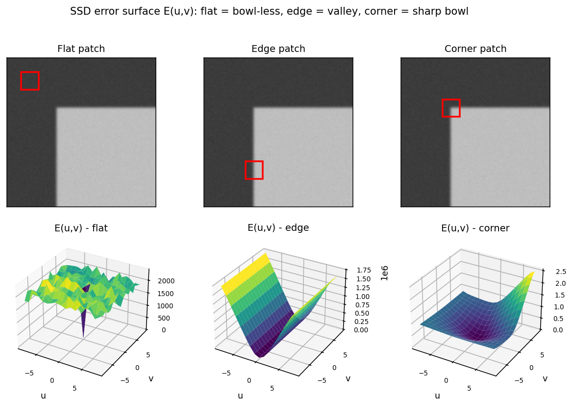
Figure 1 — SSD error surface E(u, v) for three patch types. Top: a synthetic image with a flat patch, an edge patch and a corner patch (red boxes). Bottom: the corresponding error surfaces. Flat → noisy near-zero plain (no constraint); edge → a valley with a flat floor along the edge direction (1-D ambiguity); corner → a sharp bowl with a unique minimum at (0, 0).
বাংলা: তিন রকম patch-এর জন্য E(u, v)-এর চেহারা: flat-এ প্রায় শূন্য সমতল (কোনো তথ্য নেই), edge-এ এক দিকে খোলা নালা (সেই দিকে match ambiguous), corner-এ চারদিক-বন্ধ খাড়া বাটি — মাঝখানের একটাই minimum, তাই corner-ই নিখুঁতভাবে মেলে।
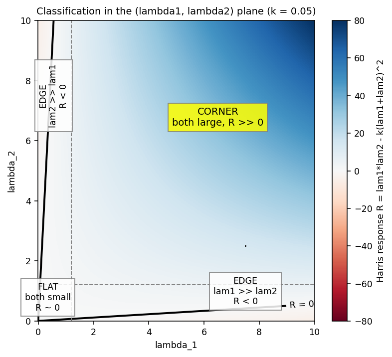
Figure 2 — classification in the (λ₁, λ₂) plane. Colour = Harris response \(R = \lambda _{1}\lambda _{2} - k(\lambda _{1}+\lambda _{2})^{2}\) (k = 0.05); the black curve is \(R = 0\). Near the origin: flat. Along either axis (one eigenvalue dominant): \(R < 0\), edge. Upper-right (both large): R ≫ 0, corner. Note the R = 0 boundary is curved — Harris's acceptance region is not the square corner that Shi–Tomasi's \(\min (\lambda ) > \tau\) would give.
বাংলা: (λ₁, λ₂)-plane-এ তিনটা অঞ্চল: origin-এর কাছে flat, যেকোনো এক অক্ষ ঘেঁষে (এক eigenvalue প্রবল) R ঋণাত্মক — edge, আর ডান-উপরে দুটোই বড় — corner, R অনেক ধনাত্মক। কালো \(R = 0\) রেখাটা বাঁকা — এখানেই Harris আর Shi–Tomasi-র সিদ্ধান্ত-অঞ্চলের পার্থক্য।
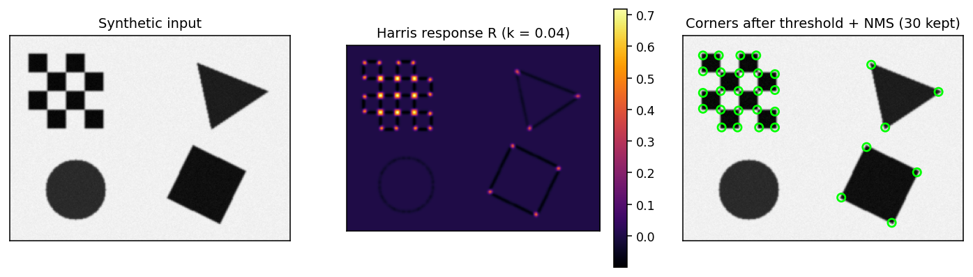
Figure 3 — Harris in action (k = 0.04). Left: synthetic scene (checkerboard, triangle, circle, rotated square). Middle: response R — bright spots exactly at corners, near-zero on flat areas, slightly negative ridges along edges. Right: keypoints after thresholding (\(R > 0.01\cdot R_\max\)) and non-max suppression. Crucial observation: the circle produces no corners (its boundary is pure edge everywhere — locally one dominant gradient direction), while every polygon vertex and checkerboard junction fires. বাংলা: বাঁয়ে কৃত্রিম দৃশ্য, মাঝে Harris response — corner-এ উজ্জ্বল বিন্দু, flat-এ শূন্য, edge বরাবর হালকা ঋণাত্মক রেখা। ডানে threshold + non-max suppression-এর পরের keypoint। সবচেয়ে শিক্ষণীয়: বৃত্তে একটাও corner নেই — বৃত্তের ধার সব জায়গাতেই শুধুই edge (স্থানীয়ভাবে এক দিকের gradient), অথচ চৌকো-ত্রিভুজের প্রতিটা কোণা আর checkerboard-এর প্রতিটা সংযোগবিন্দু ধরা পড়েছে।
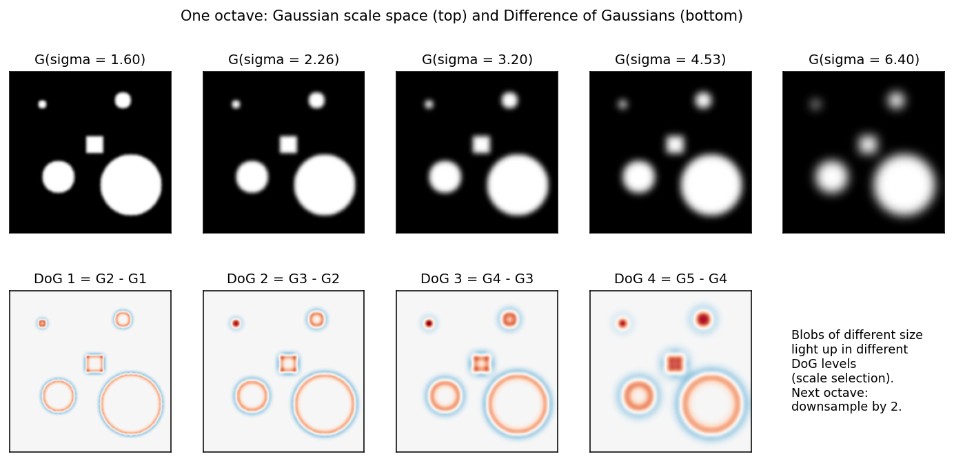
Figure 4 — one octave of scale space and its DoG stack. Top: the same blob image blurred with σ = 1.60, 2.26, 3.20, 4.53, 6.40 (factor √2). Bottom: differences of adjacent levels. Small blobs respond strongest in early DoG levels, large blobs in later ones — each structure "lights up" at its own characteristic scale. When σ has doubled, the image is downsampled by 2 and the next octave begins. বাংলা: একই ছবি ক্রমে বড় σ দিয়ে blur (উপরের সারি), পাশাপাশি দুটোর বিয়োগফল = DoG (নিচের সারি)। ছোট blob আগের DoG-স্তরে জ্বলে ওঠে, বড় blob পরের স্তরে — প্রতিটা কাঠামো তার নিজের characteristic scale-এ সাড়া দেয়। σ দ্বিগুণ হলে ছবি অর্ধেক করে পরের octave শুরু — এটাই Gaussian pyramid-এর সাশ্রয়।
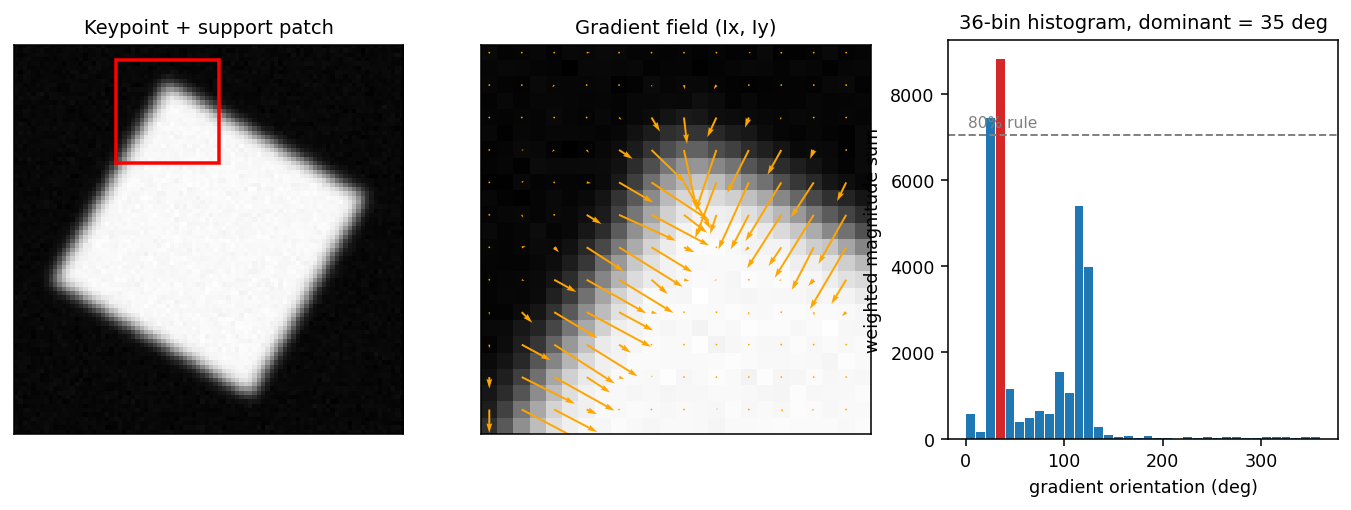
Figure 5 — dominant orientation from the 36-bin histogram. Left: keypoint at a corner of a rotated square with its support patch. Middle: the gradient field — arrows point across the two edges. Right: gradient orientations pooled into 36 bins of 10°, weighted by magnitude and a Gaussian distance weight; the red bin is the dominant orientation, the dashed line marks the 80% rule (any other bin above it would spawn a second keypoint orientation — here the second edge's peak stays below it). বাংলা: keypoint-এর চারপাশের gradient-গুলোর দিক ৩৬টা bin-এ (প্রতি bin 10°) জমা হয়, প্রতিটা vote magnitude আর দূরত্ব-Gaussian দিয়ে ওজন করা। সর্বোচ্চ (লাল) bin-টাই dominant orientation — descriptor এই দিকের সাপেক্ষে বানানো হয় বলেই SIFT rotation-invariant। dashed রেখাটা 80% rule: অন্য কোনো bin এর ওপরে গেলে সেই দিকেও আলাদা একটা keypoint বানানো হয়।
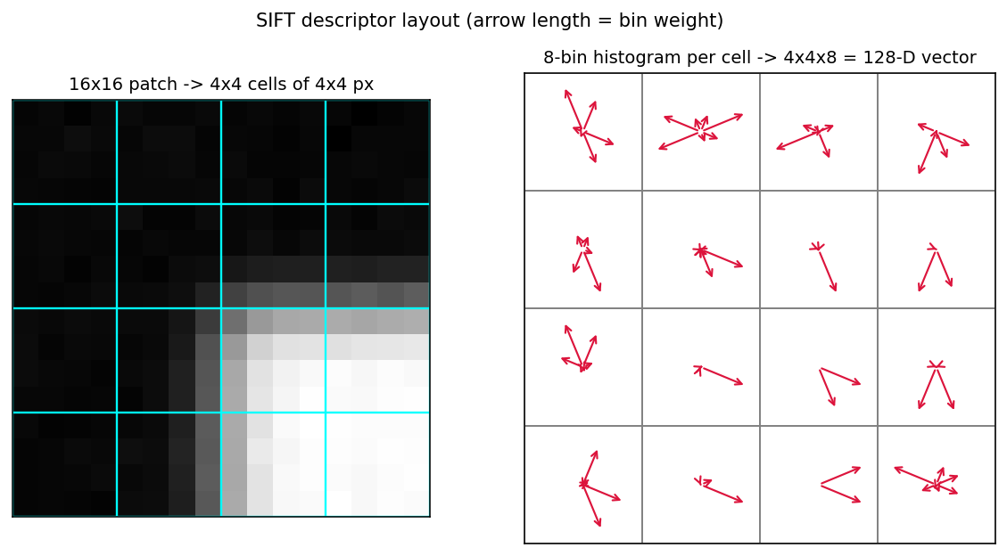
Figure 6 — the 128-D descriptor layout. Left: real 16×16 patch at a corner, divided into 4×4 cells of 4×4 pixels. Right: per cell, an 8-bin orientation histogram drawn as 8 arrows (length = bin weight). Reading off all bins: 4 × 4 × 8 = 128 numbers. The spatial grid keeps where gradients live (distinctiveness); the per-cell pooling forgives small misalignments (robustness). বাংলা: 16×16 patch-কে 4×4 cell-এ ভাগ করে প্রতি cell-এ ৮ দিকের histogram — তীরের দৈর্ঘ্য = সেই দিকের মোট gradient-ওজন। সব মিলিয়ে 4×4×8 = ১২৮টা সংখ্যা। Cell-ভাগ থাকায় কোন gradient কোথায় আছে সেই মোটা তথ্য রক্ষা পায় (distinctive), আবার cell-এর ভেতরে exact অবস্থান হারিয়ে যায় বলে সামান্য নড়চড়-বিকৃতিতেও descriptor প্রায় একই থাকে (robust)।
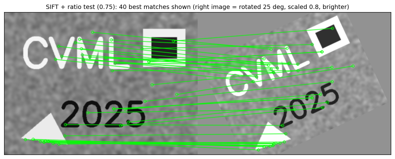
Figure 7 — SIFT matching across rotation + scale + brightness. Right image = left image rotated 25°, scaled to 0.8 and brightened; the 40 best ratio-test (0.75) matches are drawn. The match lines consistently connect the same letters/shapes despite the transformation — practical proof of SIFT's rotation, scale and illumination robustness. বাংলা: ডানের ছবিটা বাঁয়েরটারই ২৫° ঘোরানো, ০.৮ গুণ ছোট আর বেশি উজ্জ্বল সংস্করণ। তবু ratio test-উত্তীর্ণ সেরা ৪০টা match ঠিকঠাক একই অক্ষর/আকৃতিকে জুড়েছে — SIFT-এর rotation, scale ও illumination সহনশীলতার হাতে-নাতে প্রমাণ।
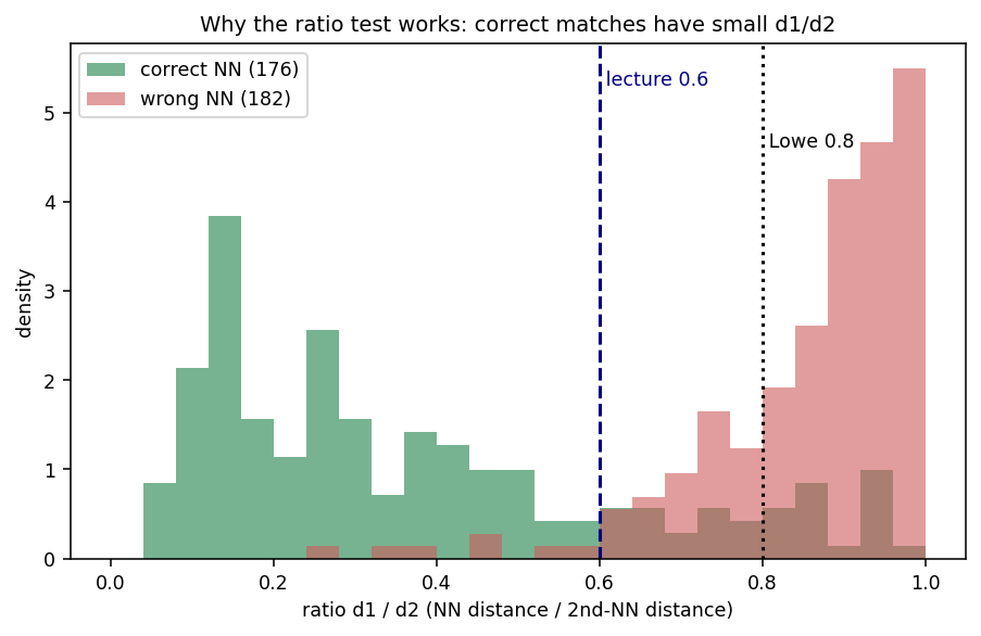
Figure 8 — why the ratio test works. For every keypoint of Figure 7 we computed \(d_{1}/d_{2}\) and checked correctness against the known ground-truth transform. Correct nearest neighbours (green) concentrate at small ratios; wrong ones (red) pile up near 1.0. The vertical lines are the two thresholds (lecture 0.6, Lowe 0.8) — both cut away almost all red while keeping most green; 0.6 is stricter (fewer false matches, also fewer correct ones). বাংলা: Figure 7-এর প্রতিটা feature-এর জন্য \(d_{1}/d_{2}\) হিসাব করে, ground-truth transform দিয়ে যাচাই করা হয়েছে match-টা সঠিক কি না। সবুজ (সঠিক) match-গুলোর অনুপাত ছোট, লাল (ভুল)-গুলো ১.০-এর কাছে স্তূপ — ঠিক Lowe-র paper-এর ছবির মতো। 0.6 বা 0.8-এ কাটলে প্রায় সব লাল বাদ যায় অথচ বেশিরভাগ সবুজ টিকে থাকে; 0.6 কড়া (ভুল কম, কিন্তু কিছু সঠিক match-ও হারায়)।
6. Algorithms & Code¶
6.1 Harris corner detector from scratch (exercise Sheet 4, task 1; cf. Ex/4/sheet4/feature_detection.py)¶
import cv2
import numpy as np

def harris_corners(gray, sigma=2.0, k=0.04, rel_tau=0.01):
    """Harris-Stephens detector. Returns corner coordinates and the response map."""
    g = gray.astype(np.float32) / 255.0
    # 1) gradients (derivative filter; the exercise uses Sobel)
    Ix = cv2.Sobel(g, cv2.CV_32F, 1, 0, ksize=3)
    Iy = cv2.Sobel(g, cv2.CV_32F, 0, 1, ksize=3)
    # 2) structure-tensor entries, smoothed with the *integration* Gaussian
    #    (the exercise sheet uses a box filter -- a Gaussian is the Harris original)
    Sxx = cv2.GaussianBlur(Ix * Ix, (0, 0), sigma)
    Syy = cv2.GaussianBlur(Iy * Iy, (0, 0), sigma)
    Sxy = cv2.GaussianBlur(Ix * Iy, (0, 0), sigma)
    # 3) response R = det(M) - k * trace(M)^2   (NO eigen-decomposition needed)
    R = (Sxx * Syy - Sxy**2) - k * (Sxx + Syy)**2
    # 4) threshold + 3x3 non-maximum suppression
    keep = (R > rel_tau * R.max()) & (R == cv2.dilate(R, np.ones((3, 3))))
    corners = np.argwhere(keep)              # array of (row, col)
    return corners, R
Key teaching points: the detection (Harris) is fully separate from any description; step 2 is where Harris improves on Shi–Tomasi (smoothing = integration Gaussian); step 3 avoids the per-pixel eigen-decomposition; step 4 turns blobs of high response into single keypoints.
বাংলা: কোডের ধাপগুলো ঠিক তত্ত্বের ধাপ: (১) Sobel দিয়ে \(I_{x}, I_{y}\); (২) তিনটা গুণফল-ছবি \(I_{x}^{2}, I_{y}^{2}, I_{x}I_{y}\) বানিয়ে integration Gaussian দিয়ে smooth — এটাই window-এর যোগফল \(\Sigma\)-এর কাজ করে; (৩) \(R = \det - k\cdot \operatorname{trace}^{2}\) — eigenvalue লাগেই না; (৪) threshold-এর সাথে dilate তুলনাটা একটা চালাক 3×3 non-max suppression: কোনো pixel-এর মান তার 3×3 প্রতিবেশের max-এর সমান হলে তবেই সে local maximum। Exercise sheet-এ Gaussian-এর বদলে box filter — দুটোই চলে, Gaussian মসৃণতর।
6.2 SIFT detection + matching with ratio test (Sheet 4, task 2)¶
sift = cv2.SIFT_create()                       # patent expired 2020 -> in main OpenCV
kp1, des1 = sift.detectAndCompute(img1_gray, None)   # keypoints + 128-D descriptors
kp2, des2 = sift.detectAndCompute(img2_gray, None)

bf = cv2.BFMatcher(cv2.NORM_L2)                # SIFT descriptors are compared with L2
knn = bf.knnMatch(des1, des2, k=2)             # the 2 nearest neighbours per query

good = [m for m, n in knn if m.distance < 0.75 * n.distance]   # Lowe ratio test

vis = cv2.drawMatches(img1, kp1, img2, kp2, good, None,
                      flags=cv2.DrawMatchesFlags_NOT_DRAW_SINGLE_POINTS)
Notes: \(k=2\) is what makes the ratio test possible (you need \(d_{2}\)); 0.75 sits between the lecture's 0.6 and Lowe's 0.8; for a panorama you would continue with cv2.findHomography(..., cv2.RANSAC) to remove the surviving outliers.
বাংলা: detectAndCompute এক ডাকে keypoint আর ১২৮-মাত্রার descriptor দুটোই দেয়। \(knnMatch(k=2)\) জরুরি — ratio test-এর জন্য দ্বিতীয় কাছের দূরত্ব \(d_{2}\) লাগবেই। List-comprehension-এর শর্তটাই Lowe-র ratio test: \(d_{1} < 0.75\cdot d_{2}\)। মনে রেখো ratio test-এর পরেও কিছু outlier টিকে থাকে — panorama বানাতে গেলে পরের ধাপে RANSAC দিয়ে homography fit করতে হয়।
6.3 ZMNCC (for trial-exam Q4b context)¶
def zmncc(W, P):
    """Zero-mean normalised cross-correlation of template W and patch P (same shape).
    Returns a value in [-1, 1]; equals the Pearson correlation coefficient."""
    Wm, Pm = W - W.mean(), P - P.mean()
    return (Wm * Pm).sum() / (np.sqrt((Wm**2).sum() * (Pm**2).sum()) + 1e-12)
বাংলা: mean বিয়োগ → dot product → দুই vector-এর দৈর্ঘ্যের গুণফল দিয়ে ভাগ — তিন লাইনেই ZMNCC। ফল −1 থেকে +1; +1 মানে নিখুঁত মিল (scale ও shift বাদে)। হরের 1e-12 শুধু শূন্য-ভাগ ঠেকাতে।
6.4 Pinhole projection (trial-exam Q4a)¶
def perspective_project(P, f):
    x, y, z = P
    return (f * x / z, f * y / z)

print(perspective_project((10, 5, 3), 2))      # -> (6.666..., 3.333...)  = (20/3, 10/3)
বাংলা: এক লাইনের হিসাব: x আর y-কে \(f/z\) দিয়ে গুণ। পরীক্ষায় ভগ্নাংশ \(20/3, 10/3\) লিখে decimal-ও দিয়ে দাও।
6.5 Pseudocode summaries (reproduce these in the exam)¶
HARRIS(I, sigma, k, tau):
  1. Ix, Iy        ← Sobel_x(I), Sobel_y(I)
  2. A, B, C       ← Gauss_sigma(Ix·Ix), Gauss_sigma(Iy·Iy), Gauss_sigma(Ix·Iy)
  3. R             ← (A·B − C²) − k·(A + B)²
  4. keypoints     ← { (x,y) : R > tau  AND  R is 3×3-local maximum }       # NMS

SIFT(I):
  1. Gaussian pyramid (octaves × scales);  DoG ← adjacent-scale differences
  2. candidates    ← extrema among 26 neighbours (3×3×3 in space-scale)
  3. refine sub-pixel (quadratic fit); reject low contrast and edge-like (Hessian ratio)
  4. orientation   ← peak of 36-bin gradient histogram (magnitude & Gaussian weighted;
                      extra keypoint for every peak ≥ 80% of max)
  5. descriptor    ← 16×16 region (rotated to orientation) → 4×4 cells × 8 bins = 128-D
  6. normalise → clip at 0.2 → renormalise

MATCH(D1, D2, t):
  for each q in D1:
      d1, d2 ← two smallest L2 distances to D2
      accept nearest neighbour iff d1 / d2 < t          # t = 0.6 (lecture) / 0.8 (Lowe)
বাংলা: এই তিনটা pseudocode মুখস্থ-সমান আয়ত্তে রাখো — Harris-এর ৪ ধাপ, SIFT-এর ৬ ধাপ, matching-এর ratio test। পরীক্ষায় "describe the algorithm" ধাঁচের প্রশ্নে এগুলোই পুরো নম্বর তোলে।
6.6 Exercise-sheet mapping (Sheet 4)¶
- Task 4.1 Harris: exactly §6.1 with \(k = 0.04\), \(\tau = 0.01\cdot R_\max\), Sobel \(ksize = 3\); visualise corners in green on the input.
- Task 4.2 SIFT matching: exactly §6.2 (\(knnMatch(k=2)\), ratio
0.75,drawMatches). - Bonus: swap in
cv2.ORB_create()(then usecv2.NORM_HAMMINGin the matcher!) and compare speed/robustness against SIFT.
বাংলা: Sheet 4-এর দুটো task উপরের দুটো code-block-ই। Bonus-এ ORB চালালে matcher-এ NORM_HAMMING দিতে ভুলো না — ORB-র descriptor binary, L2 নয়।
7. Trial-Exam Mapping¶
| Trial-exam item | Answer location | Quick answer |
|---|---|---|
| Q4a Project \(p = (10, 5, 3)\) with \(f = 2\) | §4.11, §6.4 | \(p' = (20/3, 10/3) \approx (6.67, 3.33)\) |
| Q4b ZMNCC invariant to intensity/colour shifts but fails in real lighting — why & what to do | §4.1 | invariance only if the change is consistent over the patch; shadows/materials/metamerism/SNR break it → per-channel ZMNCC, grayscale, HSV-like spaces, gradient descriptors |
| Q4c Five T/F on Harris & SIFT | table below | — |
The five T/F statements with reasoning:
| Statement | Answer | Why |
|---|---|---|
| "The elements in the diagonal of the Harris matrix control the shear and the rotation." | False | The diagonals \(\Sigma I_{x}^{2}\), \(\Sigma I_{y}^{2}\) scale the ellipse along the axes (gradient energy per axis). It is the off-diagonal \(\Sigma I_{x}I_{y}\) that controls shear/rotation — if non-zero, the ellipse axes tilt (diagonal edge or corner). |
| "A good image feature should have strong gradients in multiple directions." | True | One direction only = edge = ambiguous along it; multiple directions = corner = unique (both eigenvalues large). |
| "Template matching needs only one template for all use cases." | False | It is neither scale- nor rotation-invariant → different sizes/orientations (and object variants) need their own templates. |
| "SIFT descriptors are robust to illumination changes." | True | Gradients ignore offsets; normalisation kills contrast scaling; clipping at 0.2 + renormalising tames non-linear lighting. |
| "For rotation and scale invariance, the gradient histogram is only useful if computed globally over the entire image." | False | The opposite: SIFT computes histograms locally (orientation histogram around the keypoint; 4×4 cells in the descriptor), relative to a locally determined dominant orientation and scale. A global histogram would discard spatial structure. |
বাংলা: Q4a = সংখ্যা বসাও (\(20/3, 10/3\)); Q4b = মূলমন্ত্র "পরিবর্তনটা patch জুড়ে একই রকম হলে তবেই ZMNCC invariant" + ৩-৪টা প্রতিকার; Q4c-র পাঁচটা True/False উপরের টেবিলেই যুক্তিসহ আছে — বিশেষ করে প্রথমটা: diagonal নয়, off-diagonal entry-ই shear/rotation নিয়ন্ত্রণ করে।
8. Mock Exam — 20 Questions¶
Four tiers, five questions each. Try everything before reading the solutions.
Tier A — Basic (A1–A5)¶
A1. Define a feature. Explain in two or three sentences why a corner is a better feature than an edge or a flat region.
A2. Write down the structure tensor (Harris matrix) M for a window W. State what each of the three distinct entries represents, and what the off-diagonal entry does to the gradient ellipse.
A3. State the Harris response formula, the typical range of k, and how the sign/magnitude of R classifies flat, edge and corner.
A4. Define scale space, octave and DoG. Why does SIFT use DoG instead of the Laplacian of Gaussian?
A5. Break the number 128 in the SIFT descriptor into its factors. What are the two final normalisation steps and what is each one for? Which distance and which test are used for matching?
Tier B — Intuition (B1–B5)¶
B1. Explain, using the gradient-scatter (ellipse) picture, why the eigenvalues of M distinguish flat / edge / corner. What does each eigenvalue measure geometrically about the error surface E(u, v)?
B2. Harris and Shi–Tomasi both look at the eigenvalues of M — yet Harris never computes them. Explain how det and trace give Harris the information it needs and why this was the design goal.
B3. Why must the Laplacian be multiplied by \(\sigma ^{2}\) before comparing responses across scales? What would go wrong without this normalisation?
B4. Why does the ratio test outperform a fixed absolute threshold on \(d_{1}\)? Explain what \(d_{2}\) represents statistically and what kind of image content drives the ratio towards 1.
B5. Two related design questions: (a) Why is the SIFT descriptor computed relative to the dominant orientation? (b) Why are the gradient histograms computed in local 4×4 cells rather than one global histogram over the patch?
Tier C — Computation (C1–C5)¶
C1. A window yields the structure tensor \(M = [[8, 2], [2, 5]]\). Compute trace, det, both eigenvalues, the Harris response for \(k = 0.04\), and the Shi–Tomasi score. Classify the point (corner / edge / flat), assuming thresholds \(\tau _{Harris} = 5\) and \(\tau _{ST} = 3\).
C2. A 4-pixel window has gradient vectors \((I_{x}, I_{y})\): \((5, 0), (-5, 0), (0, 1), (0, -1)\) (box weights \(w = 1\)). Build M, compute the eigenvalues and the Harris response (\(k = 0.04\)), and classify the point. Check the consistency of your classification with the eigenvalue-ratio rule from §4.5.
C3. Query descriptor \(q = (1, 2, 0, 2)\). The two nearest candidates in the other image are \(N_{1} = (1, 1, 0, 2)\) and \(N_{2} = (1, 2, 2, 0)\). (a) Compute both L2 distances and the ratio; decide for thresholds 0.6 and 0.8. (b) A second query has \(d_{1} = 3.0, d_{2} = 3.3\); its \(d_{1}\) is larger than in case (a). What does the ratio test decide, and what lesson about absolute distances does this illustrate?
C4. For \(M = [[12, 0], [0, 2]]\): compute \(\min (\lambda _{1}, \lambda _{2})\) and the Harris R (\(k = 0.04\)). With \(\tau _{ST} = 4\) and \(\tau _{Harris} = 10\), show that the two detectors disagree, and explain in one sentence why such disagreements are possible.
C5. A 5×5 image has identical rows 0 0 9 9 9. The reference window is the 2×2 block at rows 1–2, cols 1–2 (values [0 9; 0 9]). Compute the SSD error E(u, v) for the four shifts \((\pm 1, 0), (0, \pm 1)\) and classify the location using the error-surface argument.
Tier D — Transfer (beyond the lecture) (D1–D5)¶
D1. Show that the Harris criterion \(R > 0\) is equivalent to an upper bound on the eigenvalue ratio \(r = \lambda _{1}/\lambda _{2}\). Derive the bound condition, compute the boundary ratio for \(k = 0.04\) and \(k = 0.06\), and explain what happens if someone chooses \(k = 0.3\).
D2. Sketch (or describe) the acceptance regions of Shi–Tomasi (\(\min (\lambda ) > \tau\)) and Harris (\(R > \tau '\)) in the (λ₁, λ₂)-plane. Why is \(\min (\lambda _{1}, \lambda _{2})\) the theoretically right criterion for a KLT-style tracker, and why did Harris choose a different function anyway?
D3. Describe the FAST detector's segment test and explain why it is so much faster than Harris. What does ORB add on top of FAST, which distance is used for ORB descriptors and why, and in which scenarios would you still prefer SIFT?
D4. Rotation-invariance proof sketches: (a) show that rotating the image by \(R_\theta\) transforms the structure tensor as \(M' = R_\theta M R_\theta ^{T}\) and conclude that the Harris response is rotation-invariant; (b) explain why measuring all descriptor angles relative to the dominant orientation makes the SIFT descriptor rotation-invariant.
D5. (a) Why exactly 4×4×8 = 128 dimensions — what breaks if you use 2×2×8 = 32 or 8×8×16 = 1024? (b) Hessian-based detectors: what is the Hessian matrix of an image, how do detectors like the Determinant-of-Hessian (used in SURF) differ from the structure tensor, and how is the LoG related to the Hessian?
Solutions¶
Tier A¶
A1. A feature is a small, distinctive image location (plus a description of its neighbourhood) that can be re-identified in other images of the same scene — it must be well distinguishable and well locatable. In a flat region, shifting a comparison window changes nothing, so the window matches everywhere; on an edge the window is unchanged when sliding along the edge, so the match is ambiguous along one direction; at a corner any shift changes the content, so the match is unique in both directions. বাংলা টেকঅ্যাওয়ে: Feature = চেনা-যায় ও আবার-খুঁজে-পাওয়া-যায় এমন বিন্দু; flat সব জায়গায় মেলে (অকেজো), edge এক রেখা বরাবর মেলে (ambiguous), corner ঠিক এক জায়গায় মেলে — তাই corner-ই সেরা।
A2.
\(\Sigma I_{x}^{2}\) and \(\Sigma I_{y}^{2}\) are the summed gradient energies along x and y — they scale the gradient ellipse along the axes. \(\Sigma I_{x}I_{y}\) is the correlation between x- and y-gradients — it controls the shear/rotation of the ellipse: when non-zero, the ellipse axes tilt, indicating a diagonal edge or a corner. (w = box or Gaussian window weights; with a Gaussian, this is the Harris–Stephens version.)
বাংলা টেকঅ্যাওয়ে: Diagonal দুটো = দুই অক্ষে gradient-শক্তি (ellipse-এর স্কেল); off-diagonal = দুই gradient-এর correlation (ellipse-এর কাত হওয়া)। True/False-এ এটা উল্টে দিলে ধরতে হবে।
A3. \(R = \det (M) - k\cdot \operatorname{trace}(M)^{2} = \lambda _{1}\lambda _{2} - k(\lambda _{1}+\lambda _{2})^{2}\), with \(k \approx 0.04-0.06\) (empirical). R large positive ⇒ corner (both eigenvalues large, det dominates); \(R < 0\) ⇒ edge (one eigenvalue dominates: det small, trace large); \(|R| \approx 0\) ⇒ flat (everything small). Detection = \(R > \tau\) plus non-maximum suppression.
বাংলা টেকঅ্যাওয়ে: \(R = \det - k\cdot \operatorname{trace}^{2}\); বড় ধনাত্মক = corner, ঋণাত্মক = edge, প্রায় শূন্য = flat; k ≈ 0.04–0.06; শেষে NMS।
A4. Scale space: the family \(L(x, y, \sigma ) = G_\sigma * I\) of progressively Gaussian-blurred images. Octave: the group of scales sharing one image resolution; after σ doubles, the image is downsampled by 2 and a new octave starts. DoG: the difference of two adjacent scale-space levels. SIFT uses DoG because (1) it is essentially free — pyramid levels are already computed, one subtraction each — and (2) by the heat equation \(\partial G/\partial \sigma = \sigma \nabla ^{2}G\), \(DoG \approx (k-1)\cdot \sigma ^{2}\nabla ^{2}G\), i.e. it approximates the scale-normalised LoG with the σ² normalisation built in. বাংলা টেকঅ্যাওয়ে: DoG = পাশাপাশি দুই blur-স্তরের বিয়োগ — প্রায় মুফতে, এবং σ²-normalized LoG-এর approximation, normalization নিজে থেকেই ভেতরে।
A5. \(128 = 4 \times 4 \times 8\): a 16×16 sample region → 4×4 spatial cells, each with an 8-bin orientation histogram. Normalisation steps: (1) scale to unit length — removes the multiplicative (contrast) illumination factor (gradients already removed additive offsets); (2) clip every component at 0.2 and renormalise — limits the influence of unreliable large gradient magnitudes caused by non-linear lighting (e.g. specular highlights). Matching: L2 (Euclidean) distance, nearest neighbour, accepted only if \(d_{1}/d_{2} < 0.6\) (lecture) or \(< 0.8\) (Lowe's paper). বাংলা টেকঅ্যাওয়ে: 128 = 4×4 cell × 8 bin; normalize (contrast দূর) → 0.2-এ clip (অরৈখিক আলোর বড় gradient ছাঁটা) → আবার normalize; মেলানো হয় L2 + ratio test-এ।
Tier B¶
B1. Plot every pixel's \((I_{x}, I_{y})\) of the window as a point. Flat: all points hug the origin → ellipse tiny in both axes → λ₁ ≈ λ₂ ≈ 0. Edge: gradients point (anti)parallel to one normal direction → cloud stretched along one line → one large, one small eigenvalue. Corner: two edge populations with different normals → cloud spread in two directions → both eigenvalues large. Geometrically, \(E(u, v) \approx [u v]M[u v]^{T}\), so along eigenvector \(v_{i}\) the error grows at rate \(\lambda _{i}\cdot \|shift\|^{2}\): each eigenvalue is the curvature of the error bowl along one principal direction. Flat = no bowl, edge = valley (one zero curvature), corner = bowl (two positive curvatures). বাংলা টেকঅ্যাওয়ে: λ মানে error-বাটির বক্রতা — এক দিকেও বক্রতা না থাকলে flat, এক দিকে থাকলে নালা (edge), দুই দিকেই থাকলে বাটি (corner)।
B2. Eigen-decomposition per pixel costs a square root, but the two symmetric functions of the eigenvalues are directly available from the matrix entries: \(\det (M) = AB - C^{2} = \lambda _{1}\lambda _{2}\) and \(\operatorname{trace}(M) = A + B = \lambda _{1} + \lambda _{2}\). The product is large only if both eigenvalues are large (exactly the Shi–Tomasi requirement), while the trace penalty subtracts cases where the sum is large but the product is not (edges). So \(R = \det - k\cdot \operatorname{trace}^{2}\) reads off "both eigenvalues large?" using only additions and multiplications — the design goal was a cheap, eigenvalue-free corner score with built-in smoothing. বাংলা টেকঅ্যাওয়ে: det = λ-দের গুণফল, trace = যোগফল — দুটোই matrix entry থেকে সরাসরি; গুণফল বড় মানেই দুটো λ-ই বড়, আর trace²-জরিমানা edge ছাঁটে। তাই eigenvalue ছাড়াই কাজ চলে।
B3. An n-th order Gaussian derivative shrinks like \(\sigma ^{-n}\) as σ grows, so the raw Laplacian (2nd order) decays like \(\sigma ^{-2}\): coarse scales would always respond more weakly (equivalently, in the lecture's formulation with windows, bigger integration windows would always accumulate bigger sums — bigger always wins one way or the other, so responses are simply not comparable). Multiplying by σ² exactly cancels the decay, making the response of the same structure equal in magnitude at its own scale across zoom levels — only then does "take the σ with maximal response" (characteristic-scale selection) make sense, and only then does the selected scale multiply correctly when the image is zoomed. বাংলা টেকঅ্যাওয়ে: σ বাড়লে ২য় derivative এমনিই \(1/\sigma ^{2}\) হারে কমে; σ² দিয়ে গুণ করলে সেই পক্ষপাত কাটে — তখনই "কোন σ-তে response সর্বোচ্চ" প্রশ্নটা অর্থবহ হয়।
B4. Descriptor distances have no universal scale: a "good" \(d_{1}\) for a richly textured patch can be numerically larger than a "bad" \(d_{1}\) for a bland patch, so no single absolute threshold works everywhere. The second-nearest distance \(d_{2}\) acts as a per-feature estimate of the distance to the background of wrong matches (the closest impostor). If the nearest neighbour is genuinely correct, it stands far in front of all impostors → \(d_{1}/d_{2}\) small. Repetitive structures (windows on a façade, checkerboards, foliage) produce several near-identical candidates → \(d_{1} \approx d_{2}\) → ratio ≈ 1 → correctly rejected as ambiguous. Empirically (Lowe; reproduced in Figure 8) the ratio distributions of correct and wrong matches are well separated around 0.6–0.8. বাংলা টেকঅ্যাওয়ে: \(d_{2}\) হলো "সবচেয়ে কাছের ভুল উত্তরের দূরত্ব"-এর আনুমানিক মাপ — তার সাপেক্ষে \(d_{1}\) ছোট মানেই match-টা সন্দেহাতীত; absolute threshold এ কাজ পারে না কারণ দূরত্বের কোনো সর্বজনীন স্কেল নেই।
B5. (a) Rotating the image rotates every gradient by the same angle, so the dominant orientation rotates identically; measuring all descriptor angles relative to it subtracts the rotation out — the stored numbers do not change. Without this, the same physical corner photographed at two camera roll angles would produce different descriptors. (b) A single global histogram would say which orientations occur but not where — a checkerboard corner and a completely different arrangement of the same edge directions would collide. The 4×4 spatial grid preserves coarse layout (distinctiveness) while pooling within each cell forgives a few pixels of misregistration (robustness). This is also the trial-exam T/F: local, not global. বাংলা টেকঅ্যাওয়ে: dominant orientation-এর সাপেক্ষে মাপা মানেই ঘূর্ণন বিয়োগ হয়ে যাওয়া; আর histogram local রাখার কারণ — global histogram "কোথায়" তথ্যটা হারিয়ে ফেলে, distinctiveness মরে যায়।
Tier C¶
C1. \(M = [[8, 2], [2, 5]]\):
trace = 13           det = 8·5 − 2·2 = 40 − 4 = 36
λ₁,₂ = 13/2 ± √(169/4 − 36) = 6.5 ± √(42.25 − 36) = 6.5 ± √6.25 = 6.5 ± 2.5
⇒  λ₁ = 9,  λ₂ = 4
Harris:      R = 36 − 0.04·13² = 36 − 6.76 = 29.24
Shi–Tomasi:  min(λ₁, λ₂) = 4
\(R = 29.24 > \tau _{Harris} = 5\) ⇒ corner; \(\min \lambda = 4 > \tau _{ST} = 3\) ⇒ corner. Both agree: corner (both eigenvalues comfortably positive, ratio only 2.25). বাংলা টেকঅ্যাওয়ে: নিয়মটা যান্ত্রিক: trace, det → λ = t/2 ± √((t/2)² − det) → R = det − k·trace²। এখানে দুই detector-ই একমত: corner।
C2. Sums: \(\Sigma I_{x}^{2} = 25 + 25 + 0 + 0 = 50\), \(\Sigma I_{y}^{2} = 0 + 0 + 1 + 1 = 2\), \(\Sigma I_{x}I_{y} = 0 + 0 + 0 + 0 = 0\):
M = ⎡50  0⎤    (diagonal ⇒ eigenvalues can be read off)   λ₁ = 50,  λ₂ = 2
    ⎣ 0  2⎦
R = det − k·trace² = 100 − 0.04·52² = 100 − 0.04·2704 = 100 − 108.16 = −8.16  < 0
Classification: edge (R negative; gradients almost exclusively horizontal). Consistency check with §4.5: the eigenvalue ratio is \(r = 25\), which exceeds the Harris cap for \(k = 0.04\) (\(r \approx 22.96\)) — so \(R < 0\) is exactly what the ratio rule predicts. (Shi–Tomasi agrees: \(\min \lambda = 2\) is tiny.) বাংলা টেকঅ্যাওয়ে: Diagonal matrix হলে eigenvalue সরাসরি diagonal-এই; অনুপাত 25 > 23-সীমা, তাই R ঋণাত্মক — edge। সূত্র আর সীমা-নিয়ম একই উত্তর দিল, এটাই sanity check।
C3. (a)
d(q, N₁) = √( 0² + (2−1)² + 0² + 0² ) = √1 = 1
d(q, N₂) = √( 0² + 0² + (0−2)² + (2−0)² ) = √8 ≈ 2.828
ratio = 1 / 2.828 ≈ 0.354
\(0.354 < 0.6 < 0.8\) ⇒ accepted under both thresholds — an unambiguous match. (b) \(ratio = 3.0/3.3 \approx 0.909\) ⇒ rejected by both. Lesson: case (b)'s \(d_{1} = 3.0\) is larger than case (a)'s \(d_{1} = 1\), yet that is not why it is rejected — it is rejected because an impostor sits almost equally close. Absolute distance alone cannot distinguish "far but unique" from "close but ambiguous"; the ratio can. বাংলা টেকঅ্যাওয়ে: ratio test ঠিক এটাই ধরে: (a)-তে দ্বিতীয় প্রার্থী বহু দূরে — নিশ্চিত match; (b)-তে দুই প্রার্থী গায়ে-গায়ে — ambiguous, বাদ। দূরত্ব ছোট-বড় নয়, ব্যবধানটাই আসল।
C4.
λ₁ = 12, λ₂ = 2  (diagonal matrix)
Shi–Tomasi:  min λ = 2  <  τ_ST = 4        ⇒ REJECT
Harris:      R = 12·2 − 0.04·(14)² = 24 − 7.84 = 16.16  >  τ_Harris = 10   ⇒ ACCEPT
Disagreement: Harris accepts, Shi–Tomasi rejects. Possible because the two scores are different functions of (λ₁, λ₂) with different level sets: Harris's product term lets a large λ₁ partially compensate a modest λ₂ (here ratio 6 is far below Harris's implicit cap ≈ 23), whereas Shi–Tomasi looks only at the weakest direction and is not impressed by λ₁ at all. বাংলা টেকঅ্যাওয়ে: Harris-এ বড় λ₁ ছোট λ₂-র ঘাটতি কিছুটা পুষিয়ে দিতে পারে; Shi–Tomasi শুধু দুর্বলতম দিকটাই দেখে। সীমানার কাছে তাই দুজনের রায় আলাদা হতে পারে।
C5. Every row is 0 0 9 9 9; reference \(W = [0 9; 0 9]\) (rows 1–2, cols 1–2).
shift (+1, 0): window = [9 9; 9 9],  diffs = [−9 0; −9 0]   ⇒ E = 81 + 81 = 162
shift (−1, 0): window = [0 0; 0 0],  diffs = [ 0 9;  0 9]   ⇒ E = 162
shift (0, +1): rows 2–3, cols 1–2 = [0 9; 0 9] = W          ⇒ E = 0
shift (0, −1): rows 0–1, cols 1–2 = [0 9; 0 9] = W          ⇒ E = 0
Horizontal shifts cost 162, vertical shifts cost zero — the error surface is a valley with a flat floor along y. The position is an edge: matching is fully ambiguous along the edge direction (the 1-D ambiguity that motivates corners — and, in Chapter 6, the aperture problem). বাংলা টেকঅ্যাওয়ে: এক দিকে E = 0 মানেই সেই দিকে window সরালেও কিছু বদলায় না — match ambiguous — এটা edge-এর সংখ্যাগত স্বাক্ষর।
Tier D¶
D1. With \(r = \lambda _{1}/\lambda _{2} \ge 1\) and \(\lambda _{2} > 0\):
Boundary for \(k = 0.04\): \(0.04(1+r)^{2} = r \Rightarrow 0.04r^{2} - 0.92r + 0.04 = 0 \Rightarrow r^{2} - 23r + 1 = 0 \Rightarrow r = (23 + \sqrt{525})/2 \approx 22.96\). For \(k = 0.06\): \(r^{2} - (44/3)r + 1 = 0 \Rightarrow r \approx 14.60\). So Harris with positive threshold implicitly demands an eigenvalue ratio below ≈ 23 (k = 0.04) or ≈ 14.6 (k = 0.06) — k is a roundness knob. Since \(r/(1+r)^{2}\) peaks at 0.25 (at \(r = 1\), perfectly round), choosing \(k = 0.3 > 0.25\) makes \(R < 0\) for every window — the detector finds nothing at all.
বাংলা টেকঅ্যাওয়ে: k আসলে "ellipse কতটা গোল হতে হবে"-র নব: k = 0.04 ⇒ অনুপাত-সীমা ≈ 23, k = 0.06 ⇒ ≈ 14.6, আর k ≥ 0.25 ⇒ কিছুই detect হবে না (গাণিতিকভাবে অসম্ভব শর্ত)।
D2. Shi–Tomasi's region \({\lambda _{1} > \tau and \lambda _{2} > \tau }\) is the axis-aligned square corner in the (λ₁, λ₂)-plane: its boundary consists of two straight lines, and acceptance depends only on the smaller eigenvalue. Harris's region \({\lambda _{1}\lambda _{2} - k(\lambda _{1}+\lambda _{2})^{2} > \tau '}\) is bounded by a curved (hyperbola-like) level set that bends away from the axes (Figure 2): near the axes R is negative however large the other eigenvalue is, but in between, a very large λ₁ can pull a point with modest λ₂ over the threshold. For a KLT tracker the update step solves a linear system with matrix M; the smallest eigenvalue controls the conditioning and the noise amplification of that solve in the worst direction — hence \(\min \lambda > \tau\) is precisely "the patch is reliably trackable in every direction" (Shi & Tomasi's "Good Features to Track"). Harris predates that analysis and chose \(\det - k\cdot \operatorname{trace}^{2}\) to avoid per-pixel eigen-decomposition (no square roots in 1988 hardware) while still rewarding two-large-eigenvalue configurations. বাংলা টেকঅ্যাওয়ে: Shi–Tomasi-র অঞ্চল চৌকো (শুধু ছোট λ দেখে), Harris-এর অঞ্চল বাঁকা; tracking-এর linear system-এর স্থিতিশীলতা ছোট λ-ই ঠিক করে বলে KLT-র জন্য min(λ) তাত্ত্বিকভাবে সঠিক, আর Harris-এর পছন্দটা ছিল হিসাব-সাশ্রয়ের জন্য।
D3. FAST examines the 16 pixels on a Bresenham circle of radius 3 around candidate p: p is a corner if there exists a contiguous arc of n pixels (typically 12, or 9 in FAST-9) all brighter than \(I_{p} + t\) or all darker than \(I_{p} - t\). Speed comes from (1) pure comparisons — no gradients, no products, no floats — and (2) early exit: testing the 4 compass pixels (1, 5, 9, 13) first rejects most non-corners after 2–3 comparisons; in practice the cascade is learned with a decision tree. ORB adds: a measure of orientation (intensity centroid of the patch gives an angle), steered/rotated BRIEF — a binary descriptor of pairwise intensity comparisons — and a pyramid for multi-scale. ORB descriptors are matched with the Hamming distance (count of differing bits) because they are bit strings — computable with XOR + popcount, orders of magnitude faster than 128-D float L2. Choose SIFT when robustness matters more than speed: strong scale changes, large viewpoint/illumination changes, matching against large databases; choose FAST/ORB for real-time video, SLAM and embedded hardware.
বাংলা টেকঅ্যাওয়ে: FAST = বৃত্তের ১৬ pixel-এ টানা উজ্জ্বল/অন্ধকার চাপ খোঁজা, শুধু তুলনা দিয়ে — তাই বিদ্যুৎগতি; ORB = FAST + orientation + binary BRIEF, মেলে Hamming distance-এ (XOR + bit গোনা)। গতি চাইলে ORB, চরম robustness চাইলে SIFT।
D4. (a) Let the rotated image be \(I'(x') = I(x)\) with \(x' = R_\theta x\). By the chain rule the gradient transforms as \(\nabla I'(x') = R_\theta \nabla I(x)\) — gradients are rotated by the same angle. The structure tensor is the windowed sum of outer products \(\Sigma w\cdot (\nabla I)(\nabla I)^{T}\), so
(the rotationally symmetric Gaussian window is unchanged by the rotation). \(M'\) is similar to M, hence has the same eigenvalues; since \(R = \lambda _{1}\lambda _{2} - k(\lambda _{1}+\lambda _{2})^{2}\) depends only on the eigenvalues, the Harris response is rotation-invariant (and the detected corner location rotates covariantly with the image). (b) Under the same rotation every gradient angle shifts by \(+\theta\), so the 36-bin histogram shifts circularly by θ and its peak — the dominant orientation — also shifts by exactly θ. The descriptor stores angles as (gradient angle − dominant orientation), and \((\phi + \theta ) - (\alpha + \theta ) = \phi - \alpha\): the θ cancels, the 128 numbers are unchanged. (In practice, up to sampling/interpolation noise.)
বাংলা টেকঅ্যাওয়ে: ঘূর্ণনে \(M' = RMR^{T}\) — similar matrix, eigenvalue একই, তাই Harris response বদলায় না; আর SIFT-এ সব কোণ dominant orientation বিয়োগ করে রাখা হয় বলে θ কেটে যায় — দুটোই এক লাইনের প্রমাণ, পরীক্ষায় লিখে দাও।
D5. (a) The descriptor size trades distinctiveness against robustness and cost. Too small (2×2×8 = 32): too little spatial/angular information — many different patches collide, matching precision collapses, especially in large databases. Too large (8×8×16 = 1024): each cell becomes tiny, so a small misregistration, viewpoint distortion or non-rigid deformation moves gradients into different cells/bins and changes the vector a lot — the descriptor overfits the exact appearance; storage and matching cost grow, and nearest-neighbour search suffers in very high dimensions. Lowe tested the grid empirically and 4×4 cells × 8 bins was the sweet spot — distinctive enough for million-image databases yet stable under ~50° of viewpoint change. (b) The Hessian of an image is the matrix of second derivatives,
— note: not the structure tensor, which sums products of first derivatives over a window. Determinant-of-Hessian detectors (e.g. SURF, which approximates det(H) with box filters on an integral image) respond to blobs — regions where the intensity surface curves in both directions — whereas Harris responds to corners of the edge structure. The trace of the Hessian is exactly the Laplacian: \(\operatorname{trace}(H_{img}) = I_{xx} + I_{yy} = \nabla ^{2}I\), so LoG/DoG blob detection is "trace of Hessian" detection, while SURF uses the determinant; σ²-normalisation applies to both across scales.
বাংলা টেকঅ্যাওয়ে: 128 হলো মাঝামাঝি মিষ্টি-বিন্দু — ছোট হলে সবাই সবার সাথে মিলে যায়, বড় হলে সামান্য বিকৃতিতেই ভেঙে পড়ে আর হিসাব ভারী হয়। আর Hessian = দ্বিতীয় derivative-এর matrix (structure tensor নয়!) — তার determinant blob ধরে (SURF), trace-ই হলো Laplacian (LoG/DoG)।
9. Cheat Sheet¶
Formulas (memorise cold)¶
SSD error:        E(u, v) = Σ w·[ I(x+u, y+v) − I(x, y) ]²  ≈  [u v]·M·[u v]ᵀ
Structure tensor: M = Σ w·⎡Iₓ²    IₓI_y⎤        (off-diagonal = shear/rotation of ellipse)
                          ⎣IₓI_y  I_y² ⎦
Eigenvalues:      λ₁,₂ = trace/2 ± √( (trace/2)² − det )
Classification:   λ₁≈λ₂≈0 flat   |   λ₁≫λ₂ edge   |   both large corner
Harris:           R = det(M) − k·trace(M)² = λ₁λ₂ − k(λ₁+λ₂)²,   k ≈ 0.04…0.06
                  R > τ corner,  R < 0 edge,  |R| ≈ 0 flat;  then 3×3 NMS
Shi–Tomasi:       min(λ₁, λ₂) > τ
NCC:              (W⃗ ∘ I⃗)/(‖W⃗‖‖I⃗‖)  — invariant to ×a
ZMNCC:            subtract means first — invariant to ×a and +b;  range [−1, 1]
Scale space:      L(x, y, σ) = G_σ * I;  octave = scales at one resolution
Norm. Laplacian:  σ²∇²L;   DoG ≈ (k−1)·σ²∇²G   (heat eq. ∂G/∂σ = σ∇²G)
SIFT descriptor:  16×16 → 4×4 cells × 8 bins = 128-D; normalise → clip 0.2 → renormalise
Orientation:      36 bins × 10°, magnitude + Gaussian weighted; extra keypoints at ≥80% peaks
Matching:         L2 nearest neighbour;  accept iff d₁/d₂ < 0.6 (lecture) / 0.8 (Lowe)
Repeatability:    r / min(n₁, n₂);   precision = correct/total;  recall = correct/true
Pinhole:          p′ = (f·pₓ/p_z, f·p_y/p_z);   (10,5,3), f=2 → (20/3, 10/3)
Facts that win T/F points¶
- Off-diagonal \(\Sigma I_{x}I_{y}\) tilts the gradient ellipse (shear/rotation); diagonals only scale it.
- Good feature = strong gradients in multiple directions (corner), not one (edge).
- Template matching is not scale/rotation-invariant → multiple templates needed.
- SIFT is illumination-robust because of normalise + clip-0.2 + renormalise (and gradients).
- SIFT histograms are local (orientation patch, 4×4 cells) — never global.
- Harris is rotation-invariant in response (\(M' = RMR^{T}\), same eigenvalues) but not scale-invariant; Harris–Laplace / DoG add scale.
- DoG is used because it is free (pyramid subtraction) and σ²-normalised automatically.
- k caps the eigenvalue ratio (~23 at k = 0.04, ~14.6 at 0.06; nothing detected for k ≥ 0.25).
- Ratio test rejects ambiguity (\(d_{1} \approx d_{2}\) at repetitive structures); RANSAC handles the rest later.
- SIFT: detector = DoG extrema (26 neighbours) + sub-pixel + contrast/edge rejection; descriptor = 128-D; patent expired 2020.
- ORB/FAST: binary, Hamming distance, real-time; SIFT: float, L2, maximal robustness.
বাংলা চিটশিট:
- মূল গল্প এক লাইনে: window সরাও → পরিবর্তন মাপো (
E) → Taylor-এMপাও → eigenvalue-এ flat/edge/corner → Harris \(\det - k\cdot \operatorname{trace}^{2}\) দিয়ে সস্তায় হিসাব → NMS → scale-এর জন্য DoG pyramid → rotation-এর জন্য dominant orientation → 128-D descriptor → L2 + ratio test-এ match। - λ মানে error-বাটির বক্রতা: শূন্য-শূন্য = flat, এক-শূন্য = edge, বড়-বড় = corner।
- \(\det = \lambda _{1}\lambda _{2}\) (দুটোই বড় হলে বড়), \(\operatorname{trace} = \lambda _{1}+\lambda _{2}\) — এই দুটো entry থেকেই আসে, eigenvalue লাগে না।
- k বড় ⇒ শর্ত কড়া (ellipse আরো গোল চাই); k ≥ 0.25 ⇒ কিছুই পাবে না।
- DoG = প্রায়-মুফতের LoG, σ² normalization built-in; characteristic scale = যেখানে response সর্বোচ্চ।
- SIFT-এর জাদু তিনটা: DoG-তে scale, dominant orientation-এ rotation, normalize+clip(0.2)-এ illumination।
- Ratio test: দ্বিতীয় সেরাটা কাছে থাকলেই সন্দেহ — বাদ; lecture 0.6, Lowe 0.8 — কোনটা ধরছ লিখে দাও।
- ZMNCC বাঁচে \(a\cdot I + b\) পর্যন্ত, কিন্তু patch-এর ভেতরে আলো অসমানভাবে বদলালে (ছায়া, highlight) মরে — প্রতিকার: per-channel, grayscale, HSV, gradient descriptor।
- Pinhole-এর উত্তরটা ready রাখো:
(10, 5, 3), \(f = 2\) ⇒ \((20/3, 10/3) \approx (6.67, 3.33)\)।
Last-second mantra: "Corner = both λ big. R = det − k·trace², k ≈ 0.04–0.06, negative = edge. DoG ≈ σ²-normalised LoG for free. SIFT = 4×4×8 = 128, normalise–clip-0.2–renormalise. Match = L2 + ratio (0.6 lecture / 0.8 Lowe). Pinhole p′ = f·p/z."