Chapter 06 — Optical Flow¶
Trial-exam weight: 10 / 110 points. In the trial exam this chapter appears as: backward warping + disocclusion (free text) and 5 True/False statements (flow-equation symmetry, specular surfaces, Lucas–Kanade in homogeneous regions, Horn–Schunck global smoothness, FlowNet limitations).
বাংলা: এই chapter-টি exam-এ 110 নম্বরের মধ্যে 10 নম্বর বহন করে। Trial exam-এ এসেছিল backward warping ও disocclusion নিয়ে লিখিত প্রশ্ন, আর 5টি True/False। অর্থাৎ definition + intuition + ছোট হাতে-কষা অঙ্ক — এই তিনটিই এখানে আসল অস্ত্র।
§1 Roadmap — What this chapter is about¶
Optical flow answers one question: for every pixel in frame t, where did it go in frame t+1? The answer is a 2-D displacement vector (u, v) per pixel — a dense flow field.
The logical chain of the whole chapter (memorize this skeleton):
- Motion field vs optical flow — what we want (true 2-D projection of 3-D motion) vs what we can measure (apparent motion of brightness patterns). They are not the same thing.
- Brightness constancy assumption — a moving scene point keeps its intensity: \(I(x+u, y+v, t+1) = I(x, y, t)\).
- Taylor linearization — for small motion this becomes one linear equation per pixel: \(I_{x}\cdot u + I_{y}\cdot v + I_{t} = 0\) (the optical flow constraint equation).
- Aperture problem — one equation, two unknowns
(u, v)⇒ locally we can only measure the normal flow (component perpendicular to the edge). - Lucas–Kanade (local) — assume constant flow in a small window ⇒ overdetermined system ⇒ least squares ⇒ the 2×2 matrix is the structure tensor (the Harris matrix!). Solvable only where both eigenvalues are large (corners = good features to track).
- Iterative refinement + coarse-to-fine pyramid — Taylor is only valid for motion < 1 pixel; warping iterations and image pyramids extend it to large motions.
- Horn–Schunck (global) — add a smoothness term and minimize one global energy
E = E_data + λ·E_smoothness; flow propagates into homogeneous regions but blurs across object boundaries. - Warping — backward (gather, bilinear lookup, streaks at disocclusions) vs forward (scatter, holes and overlaps). Optical flow pipelines use backward warping.
- Learning-based flow — FlowNet / FlowNet 2.0 and the modern line (LiteFlowNet2, RAFT/SEA-RAFT, GMA, FlowFormer, GMFlow, self-supervised AutoFlow).
বাংলা: পুরো chapter-এর গল্পটা একটা চেইন: আমরা চাই প্রতিটি pixel-এর displacement vector (u, v)। শুরু হয় brightness constancy assumption দিয়ে — "একটা point নড়লেও তার উজ্জ্বলতা একই থাকে"। Taylor expansion করলে পাই একটাই linear equation: I_x·u + I_y·v + I_t = 0। কিন্তু unknown দুটো (u আর v), equation একটা — তাই aperture problem। সমাধান দুই পথে: (১) Lucas–Kanade — ছোট window-র সব pixel-এ flow same ধরে নিয়ে least squares; এতে যে 2×2 matrix আসে সেটা-ই Harris-এর structure tensor। (২) Horn–Schunck — পুরো ছবির ওপর একটা global energy minimize করা, যেখানে smoothness term টেক্সচারহীন জায়গাতেও flow ছড়িয়ে দেয়। বড় motion-এর জন্য pyramid (coarse-to-fine) আর iterative warping লাগে। শেষে আসে neural network দিয়ে flow শেখা — FlowNet থেকে RAFT পর্যন্ত।
§2 Concepts from Zero¶
2.1 What is a flow field?¶
Watch a video. Between two consecutive frames, every pixel "moves" a little. Draw an arrow at every pixel saying "this brightness pattern moved from here to there" — the arrow at pixel (x, y) is the flow vector (u, v), and the full grid of arrows is the flow field. It is dense (one vector per pixel), unlike feature matching which is sparse (one vector per detected feature).
বাংলা: ভিডিওর পরপর দুটি frame নিন। প্রতিটি pixel-এ একটা তীর আঁকুন — "এই pixel-এর pattern এখান থেকে ওখানে গেছে"। pixel (x, y)-এর তীরটিই flow vector (u, v), আর সব pixel-এর তীর মিলে flow field। এটি dense — প্রতিটি pixel-এর জন্য একটি করে vector; feature matching-এর মতো sparse নয়।
2.2 Motion field vs optical flow (the rotating sphere thought experiment)¶
- Motion field = the true 2-D projection of the 3-D motion of scene points onto the image plane. This is what we would ideally like to know.
- Optical flow = the apparent motion of brightness patterns in the image. This is the only thing we can actually compute from pixel values.
The lecture's classic thought experiment: a perfectly uniform, diffuse sphere (like a ball covered in matte red paper):
- The sphere rotates about its vertical axis, lighting fixed → every scene point moves, so the motion field is non-zero. But the image looks identical in every frame (no texture, shading unchanged) → the optical flow is zero.
- The sphere is still, but the light source moves → no scene point moves, so the motion field is zero. But the highlight/shading sweeps across the image → the optical flow is non-zero.
So optical flow ≠ motion field in general. Luckily, structure usually dominates illumination in real scenes, so optical flow is a reasonable approximation of the motion field most of the time.
A second ambiguity: a point moving along its viewing ray (straight towards/away from the camera center) produces zero apparent motion — many different 3-D motions project to the same 2-D displacement. Apparent motion is only an approximation of real motion.
বাংলা: Motion field হলো scene-এর আসল 3D motion-এর image plane-এ projection — যেটা আমরা চাই। Optical flow হলো brightness pattern-এর আপাত (apparent) motion — যেটা আমরা pixel দেখে মাপতে পারি। বিখ্যাত উদাহরণ: টেক্সচারবিহীন diffuse গোলক ঘুরছে → আসল motion আছে কিন্তু ছবিতে কিছুই বদলায় না, তাই optical flow = 0। আবার গোলক স্থির কিন্তু আলো নড়ছে → আসল motion নেই, কিন্তু highlight সরে যাওয়ায় optical flow ≠ 0। অর্থাৎ দুটো এক জিনিস নয়; বাস্তবে texture সাধারণত আলোর চেয়ে শক্তিশালী বলে optical flow মোটামুটি motion field-এর কাছাকাছি থাকে। আরেকটা ambiguity: কোনো point ক্যামেরার viewing ray বরাবর সরলে image-এ কোনো displacement দেখা যায় না।
2.3 Brightness constancy — the founding assumption¶
To match a pixel between frames we need something that stays the same. The assumption: the intensity (or color) of a scene point does not change as it moves — valid for diffuse (Lambertian) materials under constant illumination. It breaks for specular (mirror-like) surfaces, moving light sources, shadows, and transparency.
বাংলা: দুই frame-এর মধ্যে pixel মেলাতে হলে এমন কিছু দরকার যা অপরিবর্তিত থাকে। ধরা হয়: একটি scene point নড়লেও তার intensity/রঙ একই থাকে — diffuse (Lambertian) surface ও স্থির আলোতে এটি সত্য। কিন্তু specular (আয়নার মতো) surface, চলমান আলো, ছায়া বা স্বচ্ছ বস্তুতে এই assumption ভেঙে যায়।
2.4 The aperture problem — why one pixel is never enough¶
Look at a moving striped pattern through a small circular hole (aperture). You can only perceive the motion component perpendicular to the stripes; any motion along the stripes is invisible because the pattern looks identical. The same happens mathematically: one pixel gives one equation with two unknowns. The classic illusion (lecture example): a rotating pole with diagonal stripes appears to move upward although the stripes physically move sideways — your brain (and plain optical flow) only senses motion along the brightness gradient.
বাংলা: ছোট গোল ছিদ্র দিয়ে চলমান ডোরাকাটা pattern দেখুন — শুধু ডোরার লম্ব দিকের motion বোঝা যায়; ডোরা বরাবর motion অদৃশ্য, কারণ pattern একই দেখায়। গাণিতিকভাবে: এক pixel = এক equation, কিন্তু unknown দুটি। লেকচারের উদাহরণ: তির্যক ডোরাকাটা ঘূর্ণায়মান খুঁটি আসলে পাশে ঘুরলেও আমাদের চোখে ওপরের দিকে উঠছে বলে মনে হয় — কারণ আমরা (এবং plain optical flow) কেবল gradient-এর দিকের motion-ই টের পাই।
2.5 Two cures: local window (LK) or global smoothness (HS)¶
- Lucas–Kanade (1981, local): assume the flow is constant inside a small window (e.g. 5×5 = 25 pixels) → 25 equations, 2 unknowns → least squares. Works only where the window contains gradients in two different directions (corners). Fails in homogeneous regions and on straight edges.
- Horn–Schunck (1981, global): assume the flow field is smooth overall → minimize one energy over the entire image = data term + λ × smoothness term. Produces flow everywhere (smoothness propagates information into textureless areas) but blurs motion boundaries.
বাংলা: Equation-এর ঘাটতি পূরণের দুই কৌশল। Lucas–Kanade (local): ছোট window-র সব pixel-এ flow একই — তাহলে ২৫টা equation, ২টা unknown → least squares। শর্ত: window-তে দুই ভিন্ন দিকের gradient থাকতে হবে (corner)। সমতল জায়গা বা সরল edge-এ fail করে। Horn–Schunck (global): পুরো flow field মসৃণ (smooth) হবে — পুরো ছবির ওপর একটাই energy minimize: data term + λ × smoothness term। টেক্সচারহীন জায়গাতেও flow পাওয়া যায়, কিন্তু object-এর সীমানায় motion ঘেঁটে (blur হয়ে) যায়।
2.6 Small motion only — pyramids to the rescue¶
The linearized flow equation comes from a first-order Taylor expansion, valid only for displacements smaller than about 1 pixel. Real videos easily contain motions of 10–50 pixels. Fix: build a Gaussian image pyramid — each level halves the resolution and therefore halves the motion. Solve flow at the coarsest level (motion now < 1 px), upsample the flow (×2 in size and ×2 in value), warp, and refine level by level. Within a level, iterative warping (warp → solve residual → add) squeezes out the remaining error.
বাংলা: Taylor expansion প্রথম order-এ কাটা হয়েছে, তাই formula কেবল ~1 pixel-এর চেয়ে ছোট motion-এ সঠিক। বাস্তবে motion হয় 10–50 pixel। সমাধান: Gaussian pyramid — প্রতি level-এ ছবি অর্ধেক হলে motion-ও অর্ধেক হয়। সবচেয়ে ছোট ছবিতে (motion < 1 px) flow বের করো, তারপর flow-কে upsample করো (আকারে ×2 এবং মানেও ×2!), warp করো, পরের level-এ refine করো। প্রতিটি level-এর ভেতরে iterative warping: warp → residual flow বের করো → যোগ করো।
2.7 Warping — using a flow field to move an image¶
Given flow from image 1 to image 2:
- Backward warping (gather): for each output pixel, look up where it came from in the source image: \(\tilde{I}(x, y) = I(x + u, y + v)\) using bilinear interpolation. No holes — every output pixel gets a value. At disocclusions (newly revealed background) it produces streaks: stretched copies of the boundary colors.
- Forward warping (scatter): push each source pixel to its destination: \(\tilde{I}(x + u, y + v) = I(x, y)\). Destinations are sub-pixel → rounding; some output pixels receive no value (holes/undefined areas, exactly at disocclusions) and some receive several (overlaps).
Optical flow pipelines (iterative LK, HS, pyramids) use backward warping because every output pixel is well defined.
বাংলা: Flow field দিয়ে ছবি সরানোর দুই পদ্ধতি। Backward warping (gather): output-এর প্রতিটি pixel-এর জন্য source ছবিতে গিয়ে দেখা "আমি কোথা থেকে এসেছি" — Ĩ(x,y) = I(x+u, y+v), bilinear interpolation দিয়ে। কোনো ফাঁকা থাকে না; disocclusion-এ (নতুন উন্মোচিত background) streak তৈরি হয় — সীমানার রঙ টেনে লম্বা হয়ে যায়। Forward warping (scatter): source-এর প্রতিটি pixel-কে গন্তব্যে ঠেলে দেওয়া — Ĩ(x+u, y+v) = I(x,y)। ফলে কিছু জায়গায় hole/undefined area (disocclusion-এ) আর কিছু জায়গায় overlap হয়। Optical flow pipeline-এ backward warping-ই standard।
2.8 Optical flow vs template matching vs feature tracking vs learning (LIVE session)¶
Task: track one object's 2-D motion through a video. Options compared in the LIVE session:
| Method | Idea | Pros / Cons |
|---|---|---|
| Template matching | slide the object patch over the next frame | simple; only rigid, non-rotating objects; fails on shape/scale/illumination change |
| Optical flow | average dense flow over object pixels | dense; small errors accumulate over time; occlusion by another object is a problem; only small displacements; homogeneous parts give false/no motion |
| Feature tracking (KLT-style) | match (SIFT) features frame-to-frame, average their motion | more robust on textured objects; needs good features and re-detection after some frames; similar background can confuse it |
| Machine learning | detect the known object class per frame | works if the class is known; needs training data |
বাংলা: একটি object-এর গতি track করার চারটি পথের তুলনা: template matching (সরল কিন্তু কেবল rigid, ঘোরে-না এমন object-এ চলে), optical flow (dense, কিন্তু ছোট ছোট error জমে accumulated drift হয়; occlusion ও texture-হীন অংশ সমস্যা; শুধু ছোট displacement), feature tracking (textured object-এ বেশি robust, কিন্তু ভালো feature লাগে ও কিছু frame পরপর নতুন feature নিতে হয়), আর machine learning (object class জানা থাকলে প্রতি frame-এ detect; training data লাগে)।
2.9 Learning optical flow — FlowNet and after¶
- FlowNet (ICCV 2015): the first CNN that regresses dense flow directly from two stacked input frames. Two variants: FlowNetSimple (frames stacked, one encoder–decoder with refinement/upconvolution) and FlowNetCorr (two separate encoders + an explicit correlation layer). Trained on the synthetic Flying Chairs dataset — and it still generalized surprisingly well, proving flow can be learned. It could not beat the classical state of the art and struggled with small motions, fine details, occlusions and real-world videos.
- FlowNet 2.0 (CVPR 2017): stacked/chained networks with warping between stages — much better quality and about 200× faster inference than classic energy-based methods of similar quality; still imperfect on fine texture and occlusions.
- Modern line (LIVE session): LiteFlowNet2 (2018; lightweight, pyramid + cascaded refinement), RAFT / SEA-RAFT (2020/2024; all-pairs correlation volume + recurrent refinement; SEA-RAFT adds direct initial-flow regression, mixture-of-Laplace loss, rigid-motion pre-training), GMA (2021; attention aggregates motion globally — helps occlusions), FlowFormer (2022; transformer over the cost volume, global context), GMFlow (2022; transformer matching with epipolar/geometry awareness), self-supervised AutoFlow (2023; no ground-truth labels — photometric consistency + smoothness + occlusion handling).
বাংলা: FlowNet (2015) প্রথম দেখায় যে দুটি frame input দিয়ে CNN সরাসরি dense flow regress করতে পারে — synthetic Flying Chairs data-তে train করেও বাস্তব ভিডিওতে মোটামুটি কাজ করে। দুর্বলতা: ছোট motion, সূক্ষ্ম detail, occlusion। FlowNet 2.0 (2017) কয়েকটি network chain করে মান অনেক বাড়ায় এবং ~200× দ্রুত। এরপর আধুনিক ধারায়: LiteFlowNet2 (হালকা-দ্রুত), RAFT/SEA-RAFT (all-pairs correlation + recurrent refinement), GMA (attention দিয়ে global motion তথ্য — occlusion-এ ভালো), FlowFormer (transformer + cost volume), GMFlow (geometry/epipolar constraint যুক্ত), AutoFlow (label ছাড়াই self-supervised training)।
2.10 Where optical flow is used (applications from the lecture)¶
- Morphing / retiming — interpolate intermediate frames along the flow (slow motion, frame-rate up-conversion).
- Video stabilization — estimate the camera-induced flow, smooth the trajectory, re-render with backward warping.
- Video editing — propagate edits/masks from one frame to the rest of a shot.
- Super-resolution — align multiple frames sub-pixel-accurately before fusing them.
- Pedestrian detection — motion is a strong cue for spotting moving people.
- Video compression — motion-compensated prediction: encode flow + small residual instead of full frames.
Also relevant context: optical flow is one of three dense-correspondence families — optical flow (no camera knowledge), stereo / multi-view reconstruction (= flow with extra constraints from known camera positions), and scene flow (stereo/multi-view plus time — the most powerful and the hardest).
বাংলা: প্রয়োগ: morphing/retiming (মাঝের frame বানানো, slow motion), video stabilization (ক্যামেরার কাঁপুনি মুছতে flow + backward warp), video editing (এক frame-এর সম্পাদনা পুরো shot-এ ছড়ানো), super-resolution (sub-pixel alignment), pedestrian detection (motion cue), video compression (flow + ছোট residual পাঠানো)। বড় চিত্রে: optical flow (ক্যামেরা অজানা) → stereo/multi-view (ক্যামেরা জানা = বাড়তি constraint) → scene flow (স্থান+সময় একসাথে — সবচেয়ে শক্তিশালী, সবচেয়ে কঠিন)।
§3 Vocabulary — Hard English Made Easy¶
| Term | Simple English | বাংলা ব্যাখ্যা | Example |
|---|---|---|---|
| Optical flow | per-pixel 2-D displacement between frames | প্রতি pixel-এর (u,v) সরণ vector — দুই frame-এর মধ্যে | dense arrows over a video frame |
| Motion field | true projection of 3-D motion onto the image | আসল 3D motion-এর image-এ projection | rotating sphere has one even if invisible |
| Apparent motion | motion you see in pixels, not in 3-D reality | pixel-এ যা নড়তে দেখা যায়, বাস্তবে নয় | moving highlight on still ball |
| Brightness constancy | a moving point keeps its intensity | নড়লেও point-এর উজ্জ্বলতা একই থাকে | I(x+u, y+v, t+1) = I(x, y, t) |
| Linearization | replace a curve by its tangent (Taylor, 1st order) | Taylor দিয়ে curve-কে সরলরেখায় approximation | flow constraint equation |
| Optical flow constraint | the one linear equation per pixel | প্রতি pixel-এ একটিমাত্র linear equation | I_x·u + I_y·v + I_t = 0 |
| Aperture problem | only motion ⊥ to the edge is locally measurable | ছোট জানালায় কেবল edge-এর লম্ব motion মাপা যায় | stripes through a hole |
| Normal flow | the measurable component along the gradient | gradient-এর দিকের measurable flow অংশ | shortest point on constraint line |
| Structure tensor | 2×2 matrix of summed gradient products (Harris matrix) | window-এ gradient গুণফলের যোগফলের 2×2 matrix | M = Σ ∇I ∇Iᵀ |
| Least squares | best fit when there are more equations than unknowns | equation বেশি, unknown কম হলে সর্বোত্তম মিল | (AᵀA)⁻¹Aᵀb |
| Eigenvalues λ₁, λ₂ | strengths of the two gradient directions in the window | window-এ দুই দিকের gradient-শক্তির মাপ | corner: both large |
| Good features to track | pixels where the structure tensor is well conditioned | যেসব pixel-এ M ভালোভাবে invertible — দুই λ-ই বড় | KLT corner selection |
| Data term | "stay faithful to the pixels" part of an energy | energy-র যে অংশ pixel-মিলকে মূল্য দেয় | (I_x u + I_y v + I_t)² |
| Smoothness term / regularizer | "keep the flow smooth" part of an energy | energy-র যে অংশ flow-এর হঠাৎ বদলকে শাস্তি দেয় | ‖∇u‖² + ‖∇v‖² |
| Euler–Lagrange equations | calculus rule to minimize an energy over a whole field | পুরো field-এর ওপর energy minimize করার নিয়ম | Horn–Schunck solver |
| Forward warping | push (scatter) source pixels to destinations | source pixel-কে গন্তব্যে ঠেলে দেওয়া (scatter) | holes + overlaps |
| Backward warping | pull (gather) a source value for each output pixel | প্রতিটি output pixel-এর জন্য source থেকে টেনে আনা (gather) | bilinear lookup, no holes |
| Bilinear interpolation | smooth value from the 4 surrounding pixels | চারপাশের ৪টি pixel মিশিয়ে sub-pixel মান | lookup at (12.3, 7.8) |
| Occlusion | a surface visible in one frame, hidden in the other | এক frame-এ দৃশ্যমান, অন্যটিতে ঢাকা পড়া অংশ | behind a moving car |
| Disocclusion | newly revealed background in the second frame | দ্বিতীয় frame-এ নতুন উন্মোচিত background | trailing edge of moving object |
| Streaks | stretched boundary colors from backward warping | backward warp-এ সীমানার রঙ টেনে লম্বা দাগ | disoccluded areas |
| Image pyramid | stack of progressively smaller, blurred images | ক্রমে ছোট ও blur করা ছবির স্তূপ | Gaussian pyramid |
| Coarse-to-fine | solve small image first, refine on larger ones | আগে ছোট ছবিতে সমাধান, পরে বড়তে refine | pyramidal LK |
| Incremental / iterative warping | warp, re-estimate residual flow, add, repeat | warp → বাকি flow বের → যোগ → আবার | flow += opticalFlow(I₁, W) |
| Specular surface | mirror-like, view-dependent appearance | আয়না-ধর্মী, দেখার কোণে রঙ বদলায় | car paint, water |
| Diffuse (Lambertian) surface | matte, same color from every viewpoint | ম্যাট — সব কোণ থেকে একই রঙ | red matte paper |
| Gradient constancy | match gradients instead of raw intensity | intensity নয়, gradient-এর মিল ধরা হয় | robust to brightness change |
| Cross-checking (left-right check) | flow forward + backward must agree, else occlusion | সামনের ও পেছনের flow না মিললে occlusion | ‖f₁₂ + f₂₁‖ > threshold |
| Correlation layer / cost volume | explicit patch-similarity computation inside a CNN | CNN-এর ভেতরে patch-মিল মাপার স্তর | FlowNetCorr, RAFT |
| Endpoint error (EPE) | average distance between estimated and true flow vectors | আনুমানিক ও আসল flow vector-এর গড় দূরত্ব | benchmark metric |
§4 Mathematical Foundations¶
4.0 Symbols used throughout¶
I(x, y, t)        image intensity at pixel (x, y) and time t,  x, y, t ∈ ℝ
(u, v)            flow vector: displacement of the pixel from frame t to t+1
I_x = ∂I/∂x       spatial derivative in x   (e.g. I(x+1,y,t) − I(x,y,t), or Sobel)
I_y = ∂I/∂y       spatial derivative in y
I_t = ∂I/∂t       temporal derivative        I(x,y,t+1) − I(x,y,t)
∇I = (I_x, I_y)ᵀ  spatial gradient
N_p / W           window (neighborhood) around pixel p
M = AᵀA           structure tensor (Harris matrix) of the window
λ₁ ≥ λ₂           eigenvalues of M
λ (or α)          smoothness weight in Horn–Schunck
বাংলা: I(x, y, t) হলো সময় t-তে (x, y) pixel-এর intensity। (u, v) হলো সেই pixel-এর displacement। I_x, I_y হলো ছবির x ও y দিকের gradient (Sobel ইত্যাদি দিয়ে মাপা যায়), আর I_t হলো একই pixel-এ দুই frame-এর intensity-র পার্থক্য। M হলো window-এর structure tensor, λ₁, λ₂ তার eigenvalue। Horn–Schunck-এ λ (অনেক বইয়ে α) smoothness-এর ওজন।
4.1 Motion field vs optical flow — formal statement¶
Motion field  m(x, y)  = projection of the 3-D velocity of the scene point
                          seen at pixel (x, y) onto the image plane
Optical flow  f(x, y)  = apparent 2-D motion of the brightness pattern at (x, y)

In general:   f ≠ m
f = m  (approximately) only when:
  • the surface is diffuse (Lambertian),
  • illumination is constant,
  • the motion is not purely along the viewing ray.
Two canonical counterexamples (exam favorites):
| Scenario | Motion field | Optical flow |
|---|---|---|
| Untextured diffuse sphere rotating about its axis, light fixed | non-zero (points really move) | zero (image never changes) |
| Static sphere, light source moves | zero (nothing moves) | non-zero (shading/highlight sweeps) |
বাংলা: Motion field হলো 3D বেগের image-এ projection (যা চাই), optical flow হলো brightness pattern-এর আপাত motion (যা মাপি)। দুটি সমান হয় কেবল diffuse surface, স্থির আলো এবং viewing ray-বরাবর-নয় এমন motion-এ। মুখস্থ রাখুন টেবিলের দুই উদাহরণ: ঘূর্ণায়মান টেক্সচারহীন গোলক → motion field ≠ 0 কিন্তু flow = 0; স্থির গোলক + চলমান আলো → motion field = 0 কিন্তু flow ≠ 0। Exam-এ এটি প্রায়ই True/False আকারে আসে।
4.2 Brightness constancy assumption¶
I(x + u, y + v, t + 1) = I(x, y, t)                 (BCA)

equivalently, with two images I₁ = frame t, I₂ = frame t+1:
I₂(x + u, y + v) = I₁(x, y)

rearranged residual form:
I(x + u, y + v, t + 1) − I(x, y, t) = 0
Meaning: the scene point that sits at (x, y) at time t has moved to (x+u, y+v) at time t+1, carrying its intensity with it unchanged. This holds for diffuse materials under constant lighting; it fails for specular surfaces, lighting changes, shadows, transparency.
বাংলা: সূত্রটির মানে — সময় t-তে (x, y)-তে থাকা scene point টি t+1-এ (x+u, y+v)-তে গেছে, আর যাওয়ার সময় তার intensity অপরিবর্তিত নিয়ে গেছে। তাই বাঁ পাশে নতুন জায়গায় নতুন সময়ের intensity, ডান পাশে পুরোনো জায়গায় পুরোনো সময়ের intensity — দুটি সমান। Diffuse surface ও স্থির আলোতে সত্য; specular surface, আলো বদল, ছায়া, স্বচ্ছতায় ভেঙে যায়।
4.3 Taylor linearization — full derivation of the constraint equation¶
Goal: turn the nonlinear equation (BCA) into something linear in (u, v).
Step 0 — recall first-order Taylor expansion in 3 variables. For a smooth function I and small increments \(\Delta x, \Delta y, \Delta t\):
Step 1 — apply it with Δx = u, Δy = v, Δt = 1 (assuming small motion, |u|, |v| < 1 px):
Step 2 — substitute into the residual form of (BCA):
Step 3 — the I(x, y, t) terms cancel:
Step 4 — equivalent forms you should recognize instantly:
I_x · u + I_y · v = − I_t                 (gradients on the left, time on the right)
∇Iᵀ · (u, v)ᵀ = − I_t                     (dot-product form)
How the derivatives are computed in practice (lecture): finite differences \(I_{x} = I(x+1, y, t) - I(x, y, t)\), \(I_{y} = I(x, y+1, t) - I(x, y, t)\), \(I_{t} = I(x, y, t+1) - I(x, y, t)\) — or better, Sobel/Prewitt filters on smoothed images.
Tiny 1-D numerical example. A 1-D edge with spatial slope \(I_{x} = 5\) gray-levels/px moves; the same pixel darkens by \(I_{t} = -10\) gray-levels between the frames. Then:
The pattern moved 2 pixels in +x direction. (In 1-D there is no aperture problem — one equation, one unknown.)
Why is this only valid for small motion? Taylor's theorem truncates the series after the linear term; the neglected remainder is \(O(u^{2} + v^{2})\) and involves second derivatives of I. If (u, v) is large, or I is strongly curved (fine texture!), the tangent-plane approximation of the image surface is wrong and the OFCE gives a wrong answer. Rule of thumb from the lecture: valid for displacements < 1 pixel.
বাংলা: Derivation-টি ধাপে ধাপে: (০) তিন চলকের Taylor expansion-এ প্রথম order পর্যন্ত রাখি। (১) Δx=u, Δy=v, Δt=1 বসাই। (২) brightness constancy-র residual রূপে বসালে (৩) I(x,y,t) দুই পাশ থেকে কেটে যায় এবং পাই I_x·u + I_y·v + I_t = 0 — এটিই optical flow constraint equation। অর্থটা সুন্দর: "spatial gradient-এর দিকে u, v পরিমাণ সরলে intensity যতটা বদলানোর কথা (I_x·u + I_y·v), সেটা temporal change (−I_t)-এর সমান হতে হবে।" এটি কেবল ছোট motion-এ (≈1 pixel-এর কম) সঠিক, কারণ Taylor-এর বাদ দেওয়া অংশ u², v²-এর মতো বাড়ে — বড় সরণে বা খুব এবড়োখেবড়ো texture-এ tangent approximation ভেঙে পড়ে। 1-D উদাহরণ: slope 5, frame-পার্থক্য −10 হলে u = 10/5 = 2 pixel।
4.4 One equation, two unknowns — aperture problem and normal flow¶
The OFCE \(I_{x}\cdot u + I_{y}\cdot v + I_{t} = 0\) is one linear equation in two unknowns (u, v). In the (u, v) plane it describes a line (the constraint line), not a point: every flow vector ending on that line satisfies the pixel's constraint perfectly. The component of the flow along the edge (perpendicular to the gradient) is completely invisible. This is the aperture problem.
What we can measure: the normal flow — the component of the flow along the gradient direction. It is the point of the constraint line closest to the origin:
                  −I_t        ∇I            −I_t · ∇I
flow_normal  =  ───────  ·  ───────   =   ─────────────
                 ‖∇I‖        ‖∇I‖            ‖∇I‖²

magnitude:  |flow_normal| = |I_t| / ‖∇I‖ ,    direction: ± ∇I/‖∇I‖
with  ‖∇I‖ = √(I_x² + I_y²)
| Symbol | Meaning |
|---|---|
| \(\nabla I = (I_{x}, I_{y})^{T}\) | spatial gradient = normal direction of the local edge |
| \(\|\nabla I\|\) | gradient magnitude (edge strength) |
| \(-I_{t}/\|\nabla I\|\) | signed speed of the pattern along the gradient |
Worked example. Let \(\nabla I = (3, 4)\), \(I_{t} = -10\).
‖∇I‖ = √(3² + 4²) = √25 = 5
normal speed   = −I_t / ‖∇I‖ = 10/5 = 2
flow_normal    = 2 · (3/5, 4/5) = (1.2, 1.6)
check: I_x·u + I_y·v = 3·1.2 + 4·1.6 = 3.6 + 6.4 = 10 = −I_t ✓
Any vector \((1.2, 1.6) + s\cdot (-4, 3)\) for arbitrary s (adding a multiple of the edge direction, which is perpendicular to \(\nabla I\)) satisfies the constraint equally well — the ambiguity is exactly one-dimensional.
বাংলা: একটি pixel একটি মাত্র linear equation দেয়, কিন্তু unknown (u, v) দুটি — তাই (u, v)-তলে সমাধান একটি বিন্দু নয়, একটি সরলরেখা (constraint line)। Edge-এর দিক বরাবর flow-এর অংশটি সম্পূর্ণ অদৃশ্য — এটিই aperture problem। যা মাপা যায় তা হলো normal flow: gradient-এর দিকে flow-এর অভিক্ষেপ, যার মান |I_t|/‖∇I‖ এবং দিক ∇I/‖∇I‖ — জ্যামিতিকভাবে এটি constraint line-এর উপর origin-এর সবচেয়ে কাছের বিন্দু। উদাহরণে ∇I=(3,4), I_t=−10 হলে ‖∇I‖=5, speed = 10/5 = 2, normal flow = (1.2, 1.6)। এর সাথে edge-direction (−4,3)-এর যেকোনো গুণিতক যোগ করলেও equation মেনে চলে — অস্পষ্টতা ঠিক এক মাত্রার।
4.5 Lucas–Kanade — local least squares and the structure tensor¶
Assumption: the flow (u, v) is constant for all pixels inside a window \(N_{p}\) around pixel p (e.g. 5×5). Each window pixel \(p_{i} = (x_{i}, y_{i})\) contributes one OFCE:
I_x(p₁)·u + I_y(p₁)·v = −I_t(p₁)
I_x(p₂)·u + I_y(p₂)·v = −I_t(p₂)
        ⋮
I_x(p_n)·u + I_y(p_n)·v = −I_t(p_n)        n = window size (e.g. 25)
In matrix form, an overdetermined system \(A f = b\):
      ┌ I_x(p₁)  I_y(p₁) ┐               ┌ −I_t(p₁) ┐
A  =  │ I_x(p₂)  I_y(p₂) │ ,   f = (u) , b = │ −I_t(p₂) │
      │    ⋮        ⋮    │         (v)       │    ⋮     │
      └ I_x(p_n)  I_y(p_n)┘               └ −I_t(p_n) ┘
A ∈ ℝⁿˣ², f ∈ ℝ², b ∈ ℝⁿ,  n ≫ 2
Least-squares formulation (equivalently: minimize the summed squared OFCE residuals over the window, which is the lecture's error function):
E(u, v) = Σ_{(x,y)∈N_p} ( I_x·u + I_y·v + I_t )²  =  ‖A f − b‖²   →  min

Setting ∂E/∂u = 0 and ∂E/∂v = 0 gives the normal equations:

AᵀA · f = Aᵀb        ⇒        f = (AᵀA)⁻¹ Aᵀ b     (if AᵀA invertible)
Write out AᵀA and Aᵀb explicitly (all sums over the window):
         ┌ Σ I_x²     Σ I_x·I_y ┐                ┌ Σ I_x·I_t ┐
AᵀA  =   │                      │ ,    Aᵀb = −   │           │
         └ Σ I_x·I_y  Σ I_y²    ┘                └ Σ I_y·I_t ┘

           M  ·  (u, v)ᵀ  =  − ( Σ I_x I_t ,  Σ I_y I_t )ᵀ
The 2×2 matrix \(M = A^{T}A = \Sigma \nabla I \nabla I^{T}\) is exactly the structure tensor — the Harris matrix from the features chapter (optionally with Gaussian weighting of the sums). Lucas–Kanade and Harris corner detection analyze the same matrix; the difference to plain block matching is that LK gives sub-pixel accuracy directly.
বাংলা: Lucas–Kanade-র মূল ধারণা: ছোট window-র সব pixel-এ flow একই — তাহলে n টি pixel মানে n টি equation, unknown মাত্র ২টি → overdetermined system A·f = b। সমাধান least squares-এ: window-জুড়ে squared residual E(u,v) = Σ(I_x u + I_y v + I_t)² minimize করলে normal equations আসে — AᵀA f = Aᵀb, অর্থাৎ f = (AᵀA)⁻¹Aᵀb। এখানে AᵀA matrix-টি খুললেই দেখা যায় এটি Σ∇I∇Iᵀ — অর্থাৎ Harris corner detector-এর structure tensor-ই! তাই "কোন pixel-এ flow নির্ভরযোগ্য" আর "কোন pixel ভালো corner" — দুটি একই প্রশ্ন। Block matching-এর সাথে পার্থক্য: LK সরাসরি sub-pixel নির্ভুলতা দেয়।
4.5.1 Complete hand-worked numerical example¶
A window contains 4 pixels with measured derivatives:
| pixel | I_x | I_y | I_t |
|---|---|---|---|
| p₁ | 1 | 0 | −2 |
| p₂ | 0 | 1 | −1 |
| p₃ | 1 | 1 | −3 |
| p₄ | 2 | 1 | −5 |
Step 1 — build A and b:
Step 2 — compute M = AᵀA element by element:
Σ I_x²    = 1² + 0² + 1² + 2² = 1 + 0 + 1 + 4 = 6
Σ I_x·I_y = 1·0 + 0·1 + 1·1 + 2·1 = 0 + 0 + 1 + 2 = 3
Σ I_y²    = 0² + 1² + 1² + 1² = 0 + 1 + 1 + 1 = 3

      ┌ 6  3 ┐
M  =  │      │
      └ 3  3 ┘
Step 3 — compute Aᵀb:
Step 4 — check invertibility and invert the 2×2 matrix:
det M = 6·3 − 3·3 = 18 − 9 = 9  ≠ 0   ⇒ invertible ✓

          1   ┌  3  −3 ┐       ┌  1/3  −1/3 ┐
M⁻¹  =   ─── ·│         │  =   │            │
          9   └ −3   6 ┘       └ −1/3   2/3 ┘
Step 5 — solve f = M⁻¹ Aᵀb:
Step 6 — verify against every original equation:
All four constraint lines pass exactly through (2, 1) — the data was consistent, so the least-squares residual is 0. With noisy data the lines would almost intersect, and LK returns the point minimizing the summed squared distance to all lines (in the residual sense).
Step 7 — eigenvalue check (is this window trustworthy?):
trace M = 6 + 3 = 9,  det M = 9
λ = ( trace ± √(trace² − 4·det) ) / 2 = ( 9 ± √(81 − 36) ) / 2 = ( 9 ± √45 ) / 2
λ₁ = (9 + 6.708)/2 ≈ 7.85 ,   λ₂ = (9 − 6.708)/2 ≈ 1.15
Both clearly > 0 ⇒ gradients span two directions ⇒ corner-like window ⇒ reliable flow.
বাংলা: হাতে-কষা উদাহরণটির সারমর্ম: ৪টি pixel-এর gradient থেকে A আর b বানাও (b-তে −I_t যায়, মাইনাস চিহ্ন ভুলবেন না!); M = AᵀA-র তিনটি entry হলো ΣI_x², ΣI_xI_y, ΣI_y²; det M = 9 ≠ 0 তাই invertible; 2×2 inversion-এর নিয়ম — কোণাকুণি উল্টাও, অন্য দুটির চিহ্ন বদলাও, det দিয়ে ভাগ করো; শেষে f = M⁻¹Aᵀb = (2, 1)। যাচাই: প্রতিটি equation-এ (2,1) বসালে মিলে যায়, অর্থাৎ চারটি constraint line-ই (2,1) বিন্দুতে ছেদ করে। Eigenvalue দুটি (≈7.85, ≈1.15) দুটোই বড় — window-টি corner-এর মতো, ফল নির্ভরযোগ্য।
4.5.2 Second worked example — noisy (inconsistent) data, residual ≠ 0¶
Real measurements never agree perfectly. Take 3 pixels:
| pixel | I_x | I_y | I_t | b = −I_t |
|---|---|---|---|---|
| p₁ | 1 | 0 | −2 | 2 |
| p₂ | 0 | 1 | −1 | 1 |
| p₃ | 1 | 1 | −2.5 | 2.5 |
(p₁ and p₂ alone would suggest \((u, v) = (2, 1)\), but p₃ says \(u + v = 2.5\) instead of 3 — noise.)
        ┌ 1  0 ┐          ┌ 2  ┐
A   =   │ 0  1 │ ,  b  =  │ 1  │
        └ 1  1 ┘          └ 2.5┘

M = AᵀA = ┌ 1+0+1  0+0+1 ┐ = ┌ 2  1 ┐ ,  det M = 4 − 1 = 3
          └ 0+0+1  0+1+1 ┘   └ 1  2 ┘

Aᵀb = ( 1·2 + 0·1 + 1·2.5 ,  0·2 + 1·1 + 1·2.5 )ᵀ = (4.5, 3.5)ᵀ

M⁻¹ = (1/3)·┌  2  −1 ┐
            └ −1   2 ┘

u = (1/3)·( 2·4.5 − 1·3.5 ) = (9 − 3.5)/3 = 5.5/3 ≈ 1.833
v = (1/3)·( −4.5 + 2·3.5 )  = ( −4.5 + 7 )/3 = 2.5/3 ≈ 0.833
Now the constraints are not met exactly — compute the residuals \(r_{i} = (A f - b)_{i}\):
p₁: 1.833 − 2          = −0.167
p₂: 0.833 − 1          = −0.167
p₃: 1.833 + 0.833 − 2.5 = +0.167
E = Σ r_i² = 3 · (1/6)² = 1/12 ≈ 0.083      (the minimum possible value)
sanity check (normal equations): Aᵀr = ( r₁ + r₃ , r₂ + r₃ )ᵀ = (0, 0)ᵀ ✓
Least squares splits the disagreement evenly: no flow vector satisfies all three lines, so LK returns the point with the smallest summed squared residual, and the residual vector is orthogonal to the columns of A (that is what \(A^{T}A f = A^{T}b\) means).
বাংলা: বাস্তব data-তে constraint line-গুলো এক বিন্দুতে মেলে না — এখানে p₃ একটু "ভুল" বলছে। Least squares তখন এমন (u, v) দেয় যাতে squared residual-এর যোগফল ন্যূনতম হয় (এখানে 1/12), আর residual vector টি A-র column-গুলির লম্ব হয় — Aᵀr = 0; এটিই normal equations-এর আসল মানে। লক্ষ করুন তিনটি ভুল সমান ±⅙ ভাগে ভাগ হয়ে গেছে।
4.5.3 When is M invertible? Eigenvalues ⇒ Harris ⇒ good features to track¶
M is symmetric positive semi-definite, so \(\lambda _{1} \ge \lambda _{2} \ge 0\). Solvability of LK is a statement about these eigenvalues:
FLAT region    : ∇I ≈ 0 everywhere in window  ⇒ λ₁ ≈ λ₂ ≈ 0
                 M ≈ 0, singular ⇒ no flow at all
EDGE           : all gradients parallel (one direction only)
                 ⇒ λ₁ large, λ₂ ≈ 0 ⇒ rank(M) = 1 ⇒ only NORMAL flow
CORNER/texture : gradients in ≥ 2 independent directions
                 ⇒ λ₁, λ₂ both large ⇒ M well-conditioned ⇒ full flow ✓
Why an edge makes M singular: if every gradient in the window is \(c_{i}\cdot (g_{x}, g_{y})\) for the same direction \((g_{x}, g_{y})\), then every row of A is a multiple of the same row vector ⇒ \(\operatorname{rank}(A) = 1\) ⇒ \(\operatorname{rank}(A^{T}A) = 1\) ⇒ \(\det M = 0\). No window size can fix this — summing more parallel gradients never creates a second direction. (This is the trial-exam T/F: "LK performs well in homogeneous regions with a big enough window" → FALSE.)
This is precisely the Harris corner criterion and the KLT "good features to track" rule (Shi–Tomasi: track only pixels with \(\min (\lambda _{1}, \lambda _{2}) > threshold\)): the pixels where optical flow is reliably computable are exactly the corners.
বাংলা: M symmetric ও positive semi-definite, তাই λ₁ ≥ λ₂ ≥ 0। তিনটি কেস মুখস্থ রাখুন — flat: gradient নেই → λ₁ ≈ λ₂ ≈ 0 → M singular → flow অসম্ভব; edge: সব gradient একই দিকে সমান্তরাল → A-র প্রতিটি সারি একই vector-এর গুণিতক → rank 1 → det M = 0 → শুধু normal flow; corner: দুই স্বাধীন দিকের gradient → দুই λ-ই বড় → পূর্ণ flow। গুরুত্বপূর্ণ: window যত বড়ই করুন, সমান্তরাল gradient যোগ করে দ্বিতীয় দিক কখনো তৈরি হয় না — তাই trial exam-এর statement টি FALSE। আর Shi–Tomasi-র "good features to track" নিয়ম (min(λ₁, λ₂) > threshold) মানে: যেখানে flow নির্ভরযোগ্য, সেগুলোই corner — Harris আর LK একই matrix-এর দুই ব্যবহার।
4.6 Iterative refinement and the coarse-to-fine pyramid¶
Problem: Taylor linearization assumes motion < 1 pixel; real motions are often tens of pixels.
Fix 1 — incremental (iterative) optical flow within one scale. Even if the first estimate is imperfect, warping \(I_{2}\) towards \(I_{1}\) reduces the remaining motion, so the next linearization is more valid:
flow ← 0
while not converged:
    W     ← backward_warp(I₂ towards I₁ using flow)
    Δflow ← opticalFlow(I₁, W)          # solve OFCE on the residual motion
    flow  ← flow + Δflow
Fix 2 — image pyramid for genuinely large motion. Downsampling an image by factor 2 also scales all displacements by ½:
If pixels move d at full resolution (level 0), then at pyramid level L
(downsampled L times by factor 2):

        d_L = d / 2^L

Required: d_L < 1  ⇒  2^L > d  ⇒  L > log₂(d)  ⇒  L_min = ⌈log₂ d⌉
Example: \(d = 24 px\) ⇒ \(\log _{2} 24 \approx 4.58\) ⇒ need \(L = 5\) downsamplings (\(24/32 = 0.75 px < 1\)). At level 4 the motion would still be \(24/16 = 1.5 px\) — too large.
Coarse-to-fine algorithm (lecture pseudocode):
build Gaussian pyramids of I₁ and I₂
flow ← 0 at coarsest level
for level = coarsest … finest:
    flow ← 2 · upsample(flow)            # grid ×2  AND  values ×2 !
    repeat (per-level iterations):
        W     ← backward_warp(I₂_level towards I₁_level using flow)
        for every pixel: build structure tensor, solve if possible
        flow  ← flow + Δflow
Two details students forget: (1) when moving one level finer, the flow values must be multiplied by 2, because a displacement of 1 px at level L+1 corresponds to 2 px at level L; (2) images must be smoothed (Gaussian) before downsampling to avoid aliasing — that is why it is a Gaussian pyramid.
Limitation (lecture): small, fast objects (e.g. a thin pole a few pixels wide moving many pixels) vanish at coarse pyramid levels, so the pyramid never sees their motion — motivation for large-displacement / SIFT-flow: initialize flow with sparse feature matches and keep them as soft constraints.
বাংলা: Taylor কেবল <1 pixel motion-এ চলে — দুটি প্রতিকার। (১) Iterative warping: প্রথম আনুমানিক flow দিয়ে I₂-কে I₁-এর দিকে warp করলে অবশিষ্ট motion ছোট হয়ে যায়; তখন আবার OFCE solve করে Δflow পাই এবং যোগ করি — কয়েক iteration-এই converge করে। (২) Pyramid: ছবি ২ গুণ ছোট করলে সব displacement-ও ২ গুণ ছোট হয়: d_L = d/2^L। d_L < 1 চাই, তাই L_min = ⌈log₂ d⌉; যেমন d=24 হলে ৫ বার downsample (24/32 = 0.75 px)। Coarse-to-fine চলার সময় দুটি জিনিস ভুলবেন না: প্রতি level-এ নামার সময় flow-এর মানও ×2 করতে হয় (ছোট ছবির 1 px = বড় ছবির 2 px), এবং downsample-এর আগে Gaussian smoothing করতে হয় (aliasing এড়াতে)। সীমাবদ্ধতা: সরু-দ্রুত object coarse level-এ মুছে যায় — তাই SIFT-flow-এ feature match দিয়ে flow-কে initialize করা হয়।
4.7 Horn–Schunck — global energy with a smoothness term¶
Instead of solving each window independently, Horn–Schunck poses one global optimization over the whole flow field (u(x,y), v(x,y)):
E(u, v) = Σ_{(x,y)∈I} ( I_x·u + I_y·v + I_t )²                       data term
        + λ · Σ_{(x,y)∈I} ( u_x² + u_y² + v_x² + v_y² )              smoothness term
                            └────────────‖∇u‖² + ‖∇v‖²────────────┘

(continuous form:  E = ∫∫ (I_x u + I_y v + I_t)² + λ( |∇u|² + |∇v|² ) dx dy)

E = E_data + λ · E_smoothness     →  min over the whole field
| Piece | Meaning |
|---|---|
| \((I_{x} u + I_{y} v + I_{t})^{2}\) | data term: penalizes violating the OFCE at each pixel (brightness constancy) |
| \(\|\nabla u\|^{2} + \|\nabla v\|^{2} = u_{x}^{2} + u_{y}^{2} + v_{x}^{2} + v_{y}^{2}\) | smoothness term (regularizer): penalizes spatial change of the flow — neighboring pixels should move alike |
| \(\lambda\) (often written \(\alpha\) or \(\alpha ^{2}\) in the literature) | trade-off weight between the two terms |
Effect of λ (qualitative — exam favorite):
- \(\lambda \to 0\): data term dominates → flow follows pixel evidence only → noisy, undefined in homogeneous regions, sharp transitions allowed (cf. LIVE-session pole example: low smoothness lets border pixels and homogeneous areas behave differently — areas around edges move in the gradient direction, homogeneous areas stay static).
- \(\lambda large\): smoothness dominates → very smooth flow, information propagates far into textureless areas (the car example: background vectors follow the car although the background has no features), but motion bleeds across object boundaries and discontinuities are blurred (pole example: high smoothness makes the whole pattern move coherently, probably upward).
Solving it — Euler–Lagrange. The minimizer of this energy must satisfy the Euler–Lagrange equations; for Horn–Schunck they are two coupled linear PDEs:
I_x (I_x u + I_y v + I_t) − λ Δu = 0
I_y (I_x u + I_y v + I_t) − λ Δv = 0          Δ = Laplace operator (u_xx + u_yy)
Discretizing \(\Delta u \approx \bar{u} - u\) (local average minus center) yields the classic Jacobi/Gauss–Seidel iteration:
        r  = ( I_x·ū + I_y·v̄ + I_t ) / ( λ + I_x² + I_y² )
        u ← ū − I_x · r
        v ← v̄ − I_y · r
(ū, v̄ = local neighborhood averages of the current u, v)
Hand-worked single iteration. Take a pixel with \(I_{x} = 1, I_{y} = 2, I_{t} = -5\), weight \(\lambda = 5\), initial flow zero (\(\bar{u} = \bar{v} = 0\)):
Interpretation: the pure constraint solution of minimum norm (the normal flow) would be \(-I_{t}\cdot \nabla I/\|\nabla I\|^{2} = 5\cdot (1,2)/5 = (1, 2)\). One HS iteration moves from (0,0) exactly the fraction \(\|\nabla I\|^{2}/(\lambda + \|\nabla I\|^{2}) = 5/10 = 1/2\) of the way towards it — the smoothness weight damps the data-driven update, and the neighborhood averages drag the result towards the neighbors over subsequent iterations. In practice HS is also run coarse-to-fine with warping per pyramid level, exactly like LK.
LK vs HS in one breath (lecture's summary): HS has a good smoothness term but basically no data aggregation (single pixel values); LK has a better data term (a whole window) but no smoothness. Modern variational methods combine both.
বাংলা: Horn–Schunck পুরো flow field-এর ওপর একটি energy minimize করে: E = E_data + λ·E_smoothness। Data term (I_x u + I_y v + I_t)² প্রতি pixel-এ brightness constancy ভাঙলে শাস্তি দেয়; smoothness term ‖∇u‖²+‖∇v‖² পাশের pixel-এর flow আলাদা হলে শাস্তি দেয় — অর্থাৎ "প্রতিবেশীরা একই রকম নড়বে"। λ ছোট হলে flow শুধু pixel-প্রমাণ মানে — হোমোজিনিয়াস জায়গায় অনির্ধারিত ও noisy, কিন্তু ধারালো সীমানা সম্ভব; λ বড় হলে flow খুব মসৃণ — feature-হীন background-ও পাশের object-এর সাথে চলতে শুরু করে (গাড়ির উদাহরণ), কিন্তু object-সীমানায় motion গড়িয়ে (blur হয়ে) যায়। Minimize করতে Euler–Lagrange equations লাগে; discretize করলে সহজ iteration: r = (I_x ū + I_y v̄ + I_t)/(λ + I_x² + I_y²), তারপর u = ū − I_x r, v = v̄ − I_y r। হাতের হিসাবে (I_x=1, I_y=2, I_t=−5, λ=5, শূন্য থেকে শুরু): r=−0.5, u=0.5, v=1.0 — যা normal flow (1,2)-এর ঠিক অর্ধেক পথ; λ যত বড়, প্রতি ধাপে data-র টান তত কম। মনে রাখুন লেকচারের তুলনা: HS-এর smoothness ভালো কিন্তু data দুর্বল (এক pixel), LK-র data ভালো (window) কিন্তু smoothness নেই — আধুনিক পদ্ধতি দুটোই মেশায়।
4.8 Warping mathematics — backward, forward, bilinear¶
Flow field convention (lecture): \(F_{1}\to _{2}(x, y) = (u, v)\).
Backward warping  :  Ĩ₁(x, y) = I₁(x + u, y + v)
   for each OUTPUT pixel (x, y): bilinear lookup in the source image
   "Where did each pixel of the output come from in the original image?"
   → always defined (no holes); can create STRETCHED areas (streaks)
     at object boundaries / disocclusions

Forward warping   :  Ĩ₁(x + u, y + v) = I₁(x, y)
   for each SOURCE pixel: scatter its value to the destination
   "Where does this source pixel go in the target?"
   → scattered data: HOLES (undefined areas) where nothing lands
     (exactly the disoccluded areas) and OVERLAPS where several land
Trial-exam answer (Q5a): with a perfect flow and interpolated values for disocclusion, forward warping leaves disoccluded areas simply undefined (holes), while backward warping fills them with streaks — stretched copies of the boundary colors, because the lookup positions of those output pixels all land in the same thin source region near the occlusion boundary. Optical flow methods use backward warping.
Bilinear interpolation (needed because x+u, y+v are sub-pixel). 1-D linear interpolation between values \(p_{1}, p_{2}\) with parameter \(\alpha \in [0, 1]\): \(f = (1-\alpha )p_{1} + \alpha p_{2}\). In 2-D, for a query at (x+s, y+t) with \(0 \le s, t < 1\):
f_b = (1 − s)·I(x, y)     + s·I(x + 1, y)          interpolate bottom row in x
f_t = (1 − s)·I(x, y + 1) + s·I(x + 1, y + 1)      interpolate top row in x
f   = (1 − t)·f_b + t·f_t                           interpolate the results in y
Worked numeric example. Query at (10.25, 20.5), i.e. \(x=10, y=20, s=0.25, t=0.5\), with pixel values \(I(10,20)=8, I(11,20)=16, I(10,21)=12, I(11,21)=20\):
বাংলা: Backward warping: output-এর প্রতিটি pixel (x,y)-এর জন্য source-এ (x+u, y+v) জায়গায় গিয়ে bilinear lookup — সব pixel-ই মান পায়, ফাঁকা থাকে না; কিন্তু disocclusion-এ সবগুলো lookup সীমানার সরু একই অঞ্চলে গিয়ে পড়ে বলে রঙ টেনে লম্বা streak হয়। Forward warping: source pixel-কে গন্তব্যে ছুঁড়ে দেওয়া — disoccluded জায়গায় কেউ এসে পড়ে না বলে hole/undefined area, আবার কোথাও একাধিক pixel পড়ে overlap। Exam-উত্তর: FW → undefined areas; BW → streaks; optical flow-এ BW-ই ব্যবহার হয়। Bilinear interpolation: sub-pixel জায়গার মান চারপাশের ৪ pixel থেকে — আগে নিচের ও উপরের সারিতে x-দিকে interpolate (f_b, f_t), পরে y-দিকে মেশানো। সংখ্যার উদাহরণ: s=0.25, t=0.5 হলে f_b=10, f_t=14, f=12।
4.9 Refinements and extensions (brief math)¶
Gradient constancy  :  ∇I(x + u, y + v, t + 1) = ∇I(x, y, t)
   matches gradients instead of intensities → robust against additive
   brightness changes (lighting), since ∂(I + c)/∂x = ∂I/∂x

Robust cost         :  replace (·)² by ρ(·)  (L1, Charbonnier, Lorentzian)
   squared error lets outliers dominate; ρ grows slower → dampened outliers

Anisotropic smoothness: smooth ALONG edges, not ACROSS them
   (anisotropic diffusion) → sharp motion boundaries

Occlusion handling  :  cross-checking / left-right check
   compute f₁₂ (1→2) and f₂₁ (2→1); pixel occluded if
   ‖ f₁₂(x) + f₂₁(x + f₁₂(x)) ‖ > threshold; optionally enforce symmetry

Layered flow        :  segment into layers, one flow per layer
Large-displacement / SIFT flow : initialize with sparse feature matches
   (soft constraints) — rescues thin fast objects that vanish in the pyramid
User-aided flow     :  manual annotation where automation fails (film industry)
Practical sensitivities listed in the lecture summary: pyramid scaling factor, data-term design (descriptor uniqueness), smoothness term (homogeneous areas + noise robustness), preprocessing to make brightness constancy valid (work on gradients, color normalization, color space), optimizer choice (simple gradient descent can hit local minima), warping both images instead of one, median filtering the flow before upsampling to remove outliers.
বাংলা: উন্নতির কৌশলগুলো এক নজরে — gradient constancy: intensity নয়, gradient মেলাও; আলো যোগ-বিয়োগ হলে gradient বদলায় না, তাই lighting change-এ robust। Robust cost ρ(·): squared error-এ outlier-রা রাজত্ব করে; ধীরে-বাড়া ρ তাদের প্রভাব কমায়। Anisotropic smoothness: edge-এর আড়াআড়ি নয়, বরাবর smooth করো — motion-সীমানা ধারালো থাকে। Occlusion: সামনে-পেছনে দুই flow cross-check; যোগফল বড় হলে pixel-টি occluded। Layered flow: আগে segment, প্রতি layer-এ আলাদা flow। SIFT flow: sparse feature match দিয়ে initialize — pyramid-এ হারিয়ে-যাওয়া সরু দ্রুত object বাঁচে। লেকচারের practical টিপস: pyramid factor, data/smoothness term-এর নকশা, preprocessing, দুই ছবিকেই warp করা, upsample-এর আগে flow-এ median filter।
§5 Visual Gallery¶
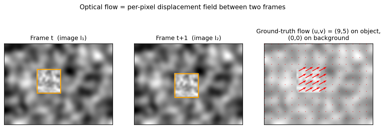
Read it like the exam: flow is defined per pixel of frame t; background pixels get (0,0), object pixels get the object's displacement. A dense field, not one global vector.
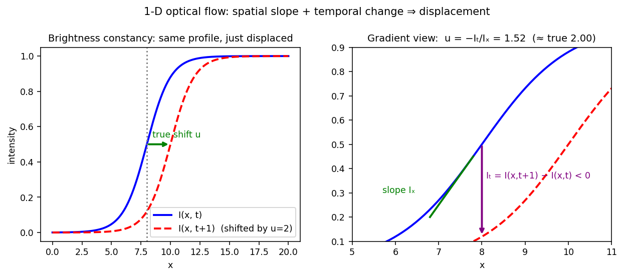
Key intuition: a steep slope means a small shift causes a big temporal change; flow estimation just divides the observed temporal change by the slope.
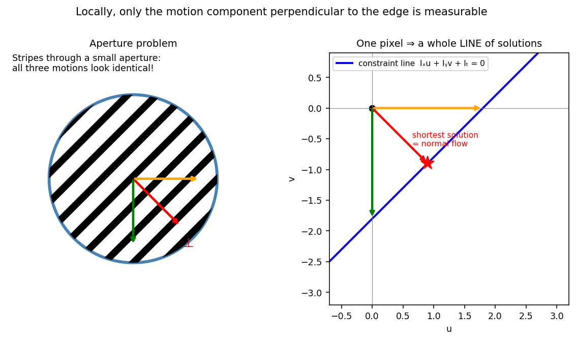
Exam phrasing: "locally, only the motion component perpendicular to the edge (along the gradient) is measurable."
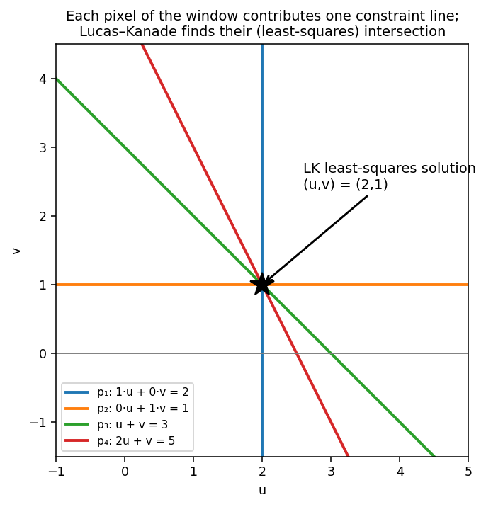
Why a window helps: one pixel = one line (ambiguous); several pixels with different gradient directions = lines with different slopes = a unique intersection. Parallel lines (an edge) never intersect in a point — that is \(\det M = 0\) drawn geometrically.
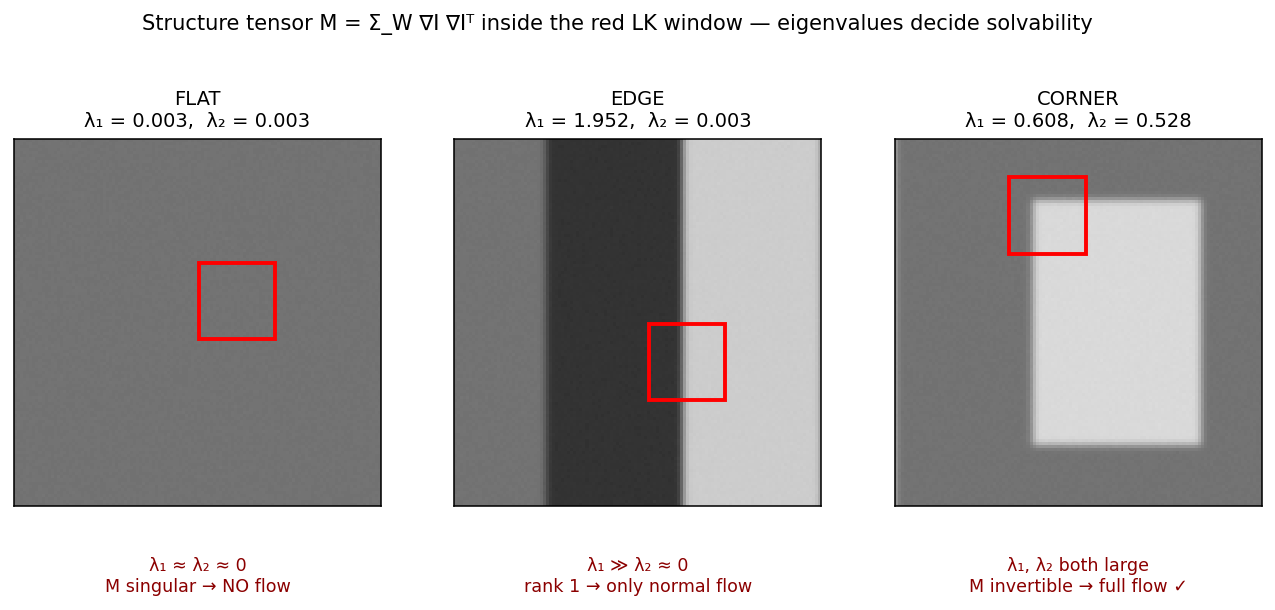
Memorize the three verdicts — they are a complete answer to "when is the LK system solvable?".
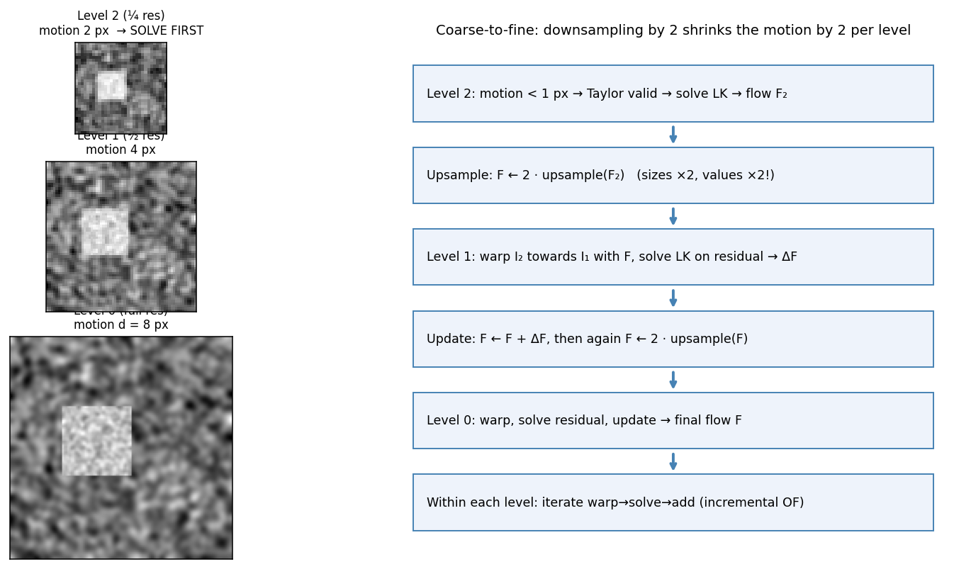
The two trap details: multiply flow values by 2 at each finer level, and Gaussian-smooth before downsampling.
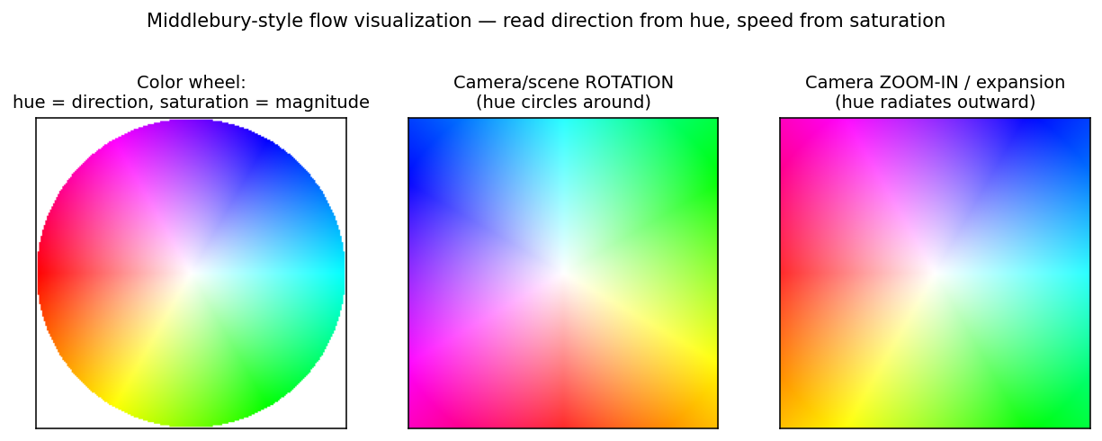
Diagnostic skill: given a colored flow image, identify translation (uniform color), rotation (hue wheel), zoom (radial hue) — a common interpretation question.
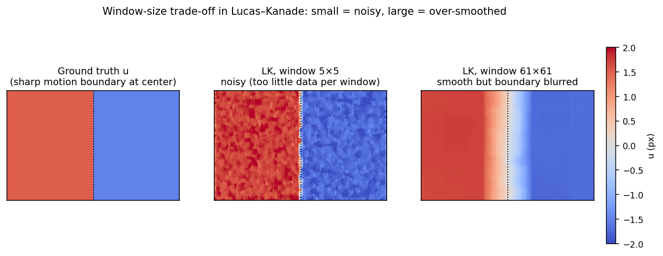
Lecture statement: too large window → edges become blurry; too small window → homogeneous regions become problematic.
§6 Algorithms & Code¶
6.1 Lucas–Kanade pseudocode (single scale)¶
For each pixel p (or each good feature):
  Build window W around p
  Compute I_x, I_y, I_t for all pixels of W (smooth first!)
  M  = [[Σ I_x², Σ I_xI_y], [Σ I_xI_y, Σ I_y²]]      # structure tensor
  b  = −[Σ I_x·I_t, Σ I_y·I_t]ᵀ
  if min eigenvalue of M > threshold:                # good feature check
      (u, v) = M⁻¹ b
  else: mark unreliable (flat/edge)
Complexity per pixel: O(|W|). Strengths: simple, parallel, sub-pixel. Weaknesses: small motion only (needs pyramid), fails on flat regions/edges.
বাংলা: প্রতি pixel-এ window নিয়ে gradient-গুলো জমাও, M আর b গড়ো, eigenvalue পরীক্ষা করে M⁻¹b solve করো। Gradient নেওয়ার আগে ছবি smooth করতে ভুলবেন না — noise সরাসরি M-এ ঢুকে যায়।
6.2 Sparse pyramidal LK with OpenCV (KLT tracking)¶
import cv2, numpy as np
prev = cv2.imread('frame1.png', cv2.IMREAD_GRAYSCALE)
curr = cv2.imread('frame2.png', cv2.IMREAD_GRAYSCALE)

# Shi-Tomasi 'good features to track' = min(λ1, λ2) criterion on the SAME
# structure tensor that LK inverts  →  track only where LK is solvable
pts0 = cv2.goodFeaturesToTrack(prev, maxCorners=200,
                               qualityLevel=0.01, minDistance=8)
pts1, status, err = cv2.calcOpticalFlowPyrLK(prev, curr, pts0, None,
                                             winSize=(21, 21), maxLevel=3)

vis = cv2.cvtColor(curr, cv2.COLOR_GRAY2BGR)
ok = status.flatten() == 1
for (x0, y0), (x1, y1) in zip(pts0[ok, 0], pts1[ok, 0]):
    cv2.line(vis, (int(x0), int(y0)), (int(x1), int(y1)), (0, 255, 0), 1)
cv2.imwrite('klt.png', vis)
বাংলা: goodFeaturesToTrack ঠিক সেই pixel-গুলো বাছে যেখানে structure tensor-এর ছোট eigenvalue-ও বড় — অর্থাৎ যেখানে LK-র 2×2 system নিরাপদে invert করা যায়। \(maxLevel=3\) মানে ৩-স্তরের pyramid, তাই ~2³ = ৮ গুণ বড় motion-ও ধরা যায়।
6.3 Dense Lucas–Kanade from scratch (NumPy)¶
import numpy as np
from scipy.ndimage import uniform_filter, gaussian_filter

def dense_lk(I1, I2, win=15, tau=1e-3):
    I1 = gaussian_filter(I1.astype(np.float64), 1.0)   # smooth BEFORE gradients
    I2 = gaussian_filter(I2.astype(np.float64), 1.0)
    Iy, Ix = np.gradient((I1 + I2) / 2)                # spatial gradients
    It = I2 - I1                                       # temporal gradient

    S  = lambda f: uniform_filter(f, win) * win * win  # window sums
    Jxx, Jxy, Jyy = S(Ix*Ix), S(Ix*Iy), S(Iy*Iy)       # structure tensor entries
    Jxt, Jyt      = S(Ix*It), S(Iy*It)                 #  Aᵀb entries (sign below)

    det = Jxx*Jyy - Jxy**2
    tr  = Jxx + Jyy
    lam_min = (tr - np.sqrt(np.maximum(tr**2 - 4*det, 0))) / 2

    u = np.where(lam_min > tau, (-Jyy*Jxt + Jxy*Jyt) / det, 0.0)   # M⁻¹·(−Aᵀ I_t)
    v = np.where(lam_min > tau, ( Jxy*Jxt - Jxx*Jyt) / det, 0.0)
    return u, v
বাংলা: এটি §4.5-এর সূত্রের হুবহু রূপায়ণ: window-sum দিয়ে M-এর তিনটি entry, Cramer-এর নিয়মে 2×2 inversion, আর lam_min > tau দিয়ে good-feature পরীক্ষা — flat/edge অঞ্চলে flow-কে 0 রাখা হয়েছে (চিহ্নিত করাই উত্তম)।
6.4 Horn–Schunck (dense, iterative)¶
import cv2
import numpy as np

def horn_schunck(I1, I2, lam=10.0, iters=100):
    I1 = I1.astype(np.float32) / 255
    I2 = I2.astype(np.float32) / 255
    Ix = cv2.Sobel((I1 + I2) / 2, cv2.CV_32F, 1, 0, ksize=3)
    Iy = cv2.Sobel((I1 + I2) / 2, cv2.CV_32F, 0, 1, ksize=3)
    It = I2 - I1
    u = np.zeros_like(I1); v = np.zeros_like(I1)
    avg = np.array([[1/12, 1/6, 1/12],
                    [1/6,  0,   1/6 ],
                    [1/12, 1/6, 1/12]], np.float32)
    for _ in range(iters):
        u_bar = cv2.filter2D(u, -1, avg)               # neighborhood averages
        v_bar = cv2.filter2D(v, -1, avg)
        r = (Ix*u_bar + Iy*v_bar + It) / (lam + Ix**2 + Iy**2)
        u = u_bar - Ix * r                             # Jacobi update (§4.7)
        v = v_bar - Iy * r
    return u, v
বাংলা: প্রতিটি iteration ঠিক §4.7-এর হাতে-কষা ধাপ: প্রতিবেশী গড় (ū, v̄) নাও, residual r হিসাব করো, gradient-এর দিকে সংশোধন করো। lam বড় করলে ফল মসৃণতর কিন্তু object-সীমানা ঝাপসা; ছোট করলে ধারালো কিন্তু noisy।
6.5 Backward warping (the exam's warping)¶
def backward_warp(img, u, v):
    """Output(x, y) = img(x + u, y + v) with bilinear interpolation. No holes."""
    h, w = img.shape[:2]
    yy, xx = np.mgrid[0:h, 0:w].astype(np.float32)
    map_x = xx + u.astype(np.float32)
    map_y = yy + v.astype(np.float32)
    return cv2.remap(img, map_x, map_y, interpolation=cv2.INTER_LINEAR,
                     borderMode=cv2.BORDER_REPLICATE)
Pure-NumPy version with explicit bilinear weights (mirrors §4.8 exactly):
def backward_warp_manual(img, u, v):
    h, w = img.shape[:2]
    yy, xx = np.mgrid[0:h, 0:w]
    sx, sy = xx + u, yy + v                     # sub-pixel source positions
    x0 = np.clip(np.floor(sx).astype(int), 0, w - 1)
    y0 = np.clip(np.floor(sy).astype(int), 0, h - 1)
    x1 = np.clip(x0 + 1, 0, w - 1)
    y1 = np.clip(y0 + 1, 0, h - 1)
    s, t = sx - np.floor(sx), sy - np.floor(sy)  # bilinear parameters
    f_b = (1 - s) * img[y0, x0] + s * img[y0, x1]
    f_t = (1 - s) * img[y1, x0] + s * img[y1, x1]
    return ((1 - t) * f_b + t * f_t).astype(img.dtype)
বাংলা: Output-এর প্রতিটি (x, y)-এর জন্য source-এ (x+u, y+v) — ভগ্নাংশ অবস্থান বলে bilinear interpolation; প্রতিটি output pixel-ই মান পায়, তাই hole নেই। manual সংস্করণে §4.8-এর f_b, f_t, f তিন ধাপ হুবহু চেনা যায়।
6.6 Forward warping (to see holes and overlaps)¶
def forward_warp(img, u, v):
    h, w = img.shape[:2]
    out = np.zeros_like(img, dtype=np.float64)
    cnt = np.zeros((h, w), dtype=np.int32)
    for y in range(h):
        for x in range(w):
            xx = int(round(x + u[y, x])); yy = int(round(y + v[y, x]))
            if 0 <= xx < w and 0 <= yy < h:
                out[yy, xx] += img[y, x]      # overlaps: accumulate
                cnt[yy, xx] += 1
    holes = cnt == 0                          # disoccluded → nothing landed here
    cnt[holes] = 1
    return (out / cnt).astype(img.dtype), holes
বাংলা: Scatter-পদ্ধতি — কোথাও একাধিক pixel পড়লে গড় নেওয়া হলো (overlap), আর holes mask-টি ঠিক disoccluded অঞ্চল দেখায়: forward warping-এ সেগুলো undefined থেকে যায়।
6.7 Coarse-to-fine wrapper (pyramidal flow)¶
def coarse_to_fine_flow(I1, I2, levels=4, solver=horn_schunck):
    pyr1, pyr2 = [I1], [I2]
    for _ in range(levels - 1):
        pyr1.append(cv2.pyrDown(pyr1[-1]))    # Gaussian blur + downsample by 2
        pyr2.append(cv2.pyrDown(pyr2[-1]))

    h, w = pyr1[-1].shape[:2]
    u = np.zeros((h, w), np.float32); v = np.zeros((h, w), np.float32)
    for L in reversed(range(levels)):
        hL, wL = pyr1[L].shape[:2]
        u = 2 * cv2.resize(u, (wL, hL))       # sizes ×2 AND values ×2 (§4.6!)
        v = 2 * cv2.resize(v, (wL, hL))
        warped = backward_warp(pyr2[L], u, v) # warp I2 towards I1
        du, dv = solver(pyr1[L], warped)      # residual flow at this level
        u, v = u + du, v + dv
    return u, v
বাংলা: cv2.pyrDown নিজে Gaussian smoothing করে — aliasing-এর ভয় নেই। সবচেয়ে গুরুত্বপূর্ণ লাইন: \(u = 2 * resize(u)\) — আকারের সাথে মানও দ্বিগুণ; এটি বাদ দিলে প্রতি level-এ flow অর্ধেক হয়ে ভুল ফল আসবে।
6.8 Flow visualization (color wheel) and a dense baseline¶
def flow_to_color(u, v):
    mag, ang = cv2.cartToPolar(u, v)
    hsv = np.zeros((*u.shape, 3), np.uint8)
    hsv[..., 0] = (ang * 180 / np.pi / 2).astype(np.uint8)   # hue = direction
    hsv[..., 1] = cv2.normalize(mag, None, 0, 255,
                                cv2.NORM_MINMAX).astype(np.uint8)  # sat = speed
    hsv[..., 2] = 255
    return cv2.cvtColor(hsv, cv2.COLOR_HSV2BGR)

# quick dense baseline built into OpenCV:
flow = cv2.calcOpticalFlowFarneback(prev, curr, None,
                                    0.5, 3, 15, 3, 5, 1.2, 0)
বাংলা: Hue = দিক, saturation/brightness = গতি — §5-এর color-wheel চিত্রের নিয়মেই। দ্রুত dense baseline দরকার হলে OpenCV-র Farnebäck পদ্ধতি এক লাইনে পাওয়া যায়।
6.9 Occlusion detection by cross-checking¶
def occlusion_mask(u12, v12, u21, v21, thresh=1.0):
    """Pixel occluded if forward + (warped) backward flow do not cancel."""
    u21w = backward_warp(u21, u12, v12)   # bring f21 to frame-1 coordinates
    v21w = backward_warp(v21, u12, v12)
    err = np.sqrt((u12 + u21w) ** 2 + (v12 + v21w) ** 2)
    return err > thresh
বাংলা: যে pixel সত্যিই দুই frame-এই দৃশ্যমান, তার সামনের flow আর (warp-করা) পেছনের flow যোগ করলে ≈ 0 হবে; বড় হলে pixel-টি occluded — লেকচারের cross-checking/left-right check।
§7 Trial-Exam Mapping¶
| Trial-exam item | Where it is covered now |
|---|---|
| Q5a Backward warping definition + how disoccluded areas look | §2.7, §4.8, §6.5, Mock Q4/Q9 |
| Q5b T/F #1 — symmetry of the flow relation | §4.2, Mock Q19 solution box |
| Q5b T/F #2 — specular surfaces suitable for flow? | §2.3, §4.1, Mock Q7 |
| Q5b T/F #3 — LK in homogeneous regions with big window | §4.5.2, Figure 5, Mock Q11/Q12 |
| Q5b T/F #4 — Horn–Schunck global smoothness | §4.7, Mock Q10/Q16 |
| Q5b T/F #5 — FlowNet on occlusions / fine texture | §2.9, Mock Q5 |
The five trial T/F with verdicts (memorize):
- "If H(x, y) = I(x+u, y+v) with (u, v) the motion at (x, y), then H(x−u, y−v) = I(x, y)." → TRUE — substitute \((x-u, y-v)\) into the first relation (with the same vector attached to that location); the relation is symmetric under shifting the evaluation point back along the flow.
- "Specular surfaces are particularly suitable for optical flow." → FALSE — highlights move with the light/viewpoint, not the surface; brightness constancy breaks.
- "LK performs well in homogeneous regions if the structure-tensor window is big enough." → FALSE — without gradients M stays (near-)singular at any window size.
- "Horn–Schunck imposes a global smoothness constraint on the flow field." → TRUE — that is the term \(\lambda \Sigma (\|\nabla u\|^{2} + \|\nabla v\|^{2})\).
- "FlowNet performs well on occlusions and fine texture." → FALSE — exactly its known weaknesses (improved later by RAFT/GMA-type models).
বাংলা: পাঁচটি True/False মুখস্থ রাখুন: (1) TRUE — সম্পর্কটি flow বরাবর পেছনে সরালে প্রতিসম; (2) FALSE — specular highlight আলো/দৃষ্টিকোণের সাথে নড়ে, surface-এর সাথে নয়; (3) FALSE — gradient না থাকলে window যত বড়ই হোক M singular; (4) TRUE — smoothness term-টিই global constraint; (5) FALSE — occlusion ও সূক্ষ্ম texture-ই FlowNet-এর দুর্বলতা।
§8 Mock Exam — 20 Questions¶
Tier A = Basic (definitions) · Tier B = Intuitive (why/explain) · Tier C = Harder (compute by hand) · Tier D = Transfer (beyond the lecture). Try all questions before reading the solutions.
Tier A — Basic (Q1–Q5)¶
Q1. State the brightness constancy assumption as a formula and in one sentence. Name one material class for which it holds and two situations where it fails.
Q2. Derive nothing — just write down the optical flow constraint equation and define every symbol in it. How many unknowns and how many equations does one pixel give?
Q3. Define the aperture problem in two sentences. Which component of the motion can be measured locally, and what is it called?
Q4. Give the formulas for backward warping and forward warping of image \(I_{1}\) with flow (u, v), and state for each whether it is a "gather" or a "scatter" operation.
Q5. Name the two classical optical-flow algorithms of 1981 and classify each as local or global. What did FlowNet (2015) demonstrate for the first time?
Tier B — Intuitive (Q6–Q10)¶
Q6. In the (u, v) plane, what geometric object does a single pixel's flow constraint describe? Explain geometrically why a window containing gradients of two different orientations makes the LK solution unique — and what happens geometrically when all gradients are parallel.
Q7. A polished car drives past a fixed camera on a sunny day. Explain two distinct reasons why the estimated optical flow on the car body may differ from the true motion field.
Q8. The barber-pole illusion: diagonal stripes on a rotating pole physically move sideways, yet appear to move upward. Explain this with the aperture problem, and predict what a Horn–Schunck algorithm with (a) very low λ and (b) very high λ would estimate (lecture LIVE discussion).
Q9. After computing a perfect flow between two frames where a foreground object moved, you backward-warp the second image to the first. Describe the appearance of the disoccluded areas and explain why they look like that. What would forward warping produce there instead?
Q10. Lucas–Kanade with a 5×5 window is noisy; with a 61×61 window it is smooth but wrong near motion boundaries. Explain both effects from the LK assumption.
Tier C — Harder, compute by hand (Q11–Q15)¶
Q11. A 2-pixel window has measurements \(p_{1}: I_{x}=2, I_{y}=0, I_{t}=-4\) and \(p_{2}: I_{x}=0, I_{y}=1, I_{t}=1\).
(a) Write the LK system \(A(u,v)^{T} = b\). (b) Check whether \(M = A^{T}A\) is invertible. © Solve for (u, v).
(d) Now replace \(p_{2}\) by \(p_{2}': I_{x}=4, I_{y}=0, I_{t}=-8\). Is M still invertible? What can you still recover?
Q12. At a pixel, \(\nabla I = (4, 3)\) and \(I_{t} = -5\). (a) Compute the normal flow vector. (b) Verify it satisfies the constraint equation. © Write the general solution set of the constraint and explain which part is unobservable.
Q13. A window contains 4 pixels: \(p_{1}: (I_{x}, I_{y}, I_{t}) = (2, 1, 0)\), \(p_{2}: (1, 0, 1)\), \(p_{3}: (0, 2, -4)\), \(p_{4}: (1, 1, -1)\). Build \(M = A^{T}A\) and \(A^{T}b\), verify invertibility, compute \(M^{-1}\) explicitly, solve for (u, v), and compute the eigenvalues of M.
Q14. Pixels in a video move up to \(d = 24 px\) between frames; your solver tolerates motion < 1 px. (a) Using a factor-2 Gaussian pyramid, derive the minimum number of downsampling steps. (b) At the coarsest valid level you estimate flow \((0.75, -0.5)\) at some pixel. What flow value does this become after transferring it one level finer, and why? © Why is the image blurred before each downsampling?
Q15. Horn–Schunck Jacobi update at a pixel: \(I_{x} = 2, I_{y} = 1, I_{t} = -10\), smoothness weight \(\lambda = 5\), current neighborhood averages \(\bar{u} = 1, \bar{v} = 1\).
(a) Compute the updated (u, v). (b) Compute the data residual \(I_{x} u + I_{y} v + I_{t}\) before and after the update and comment. © What happens to the update step as \(\lambda \to \infty\)?
Tier D — Transfer, beyond the lecture (Q16–Q20)¶
Q16. Compare Horn–Schunck's global smoothness with Lucas–Kanade's local constancy as two different priors that resolve the same underdetermination. For each prior, give one scene where it is the better model and one where it fails. Sketch how a modern method could combine both (lecture hint: HS has a good smoothness term but a weak data term; LK the opposite).
Q17. A perfectly uniform, diffuse (matte) sphere rotates about its vertical axis under fixed lighting; a camera films it. (a) What is the motion field? (b) What optical flow will any brightness-based algorithm estimate, and why? © Now keep the sphere still and move the lamp — what happens to each quantity? (d) What do these cases prove about optical flow as a measurement of motion?
Q18. A drone video contains displacements of 40+ pixels between frames. (a) Explain precisely which mathematical step of the derivation breaks. (b) Explain how the coarse-to-fine pyramid repairs it, including the formula for the motion at level L. © Give one failure case of the pyramid strategy itself and the lecture's remedy for it.
Q19. Between two frames, the camera's automatic exposure brightens the whole second image by 20 gray-levels (no scene motion at all). (a) What flow does the OFCE predict at a pixel with \(\nabla I = (5, 0)\)? Compute it. (b) Why is this flow wrong? © Name and write the modified constancy assumption that fixes this, and explain why it works.
Q20. Explain the relationship between Lucas–Kanade flow, the KLT feature tracker, and Harris/Shi–Tomasi corner detection: which matrix do they share, what criterion does "good features to track" impose on it, and why does the LIVE session recommend feature tracking over raw optical flow for tracking an object across many frames?
Solutions¶
Tier A solutions¶
S1. Formula: \(I(x + u, y + v, t + 1) = I(x, y, t)\) (equivalently \(I_{2}(x+u, y+v) = I_{1}(x, y)\)). Sentence: a scene point keeps its intensity (color) while it moves between frames. Holds for diffuse (Lambertian) materials under constant illumination. Fails for: specular surfaces (highlights move with light/viewpoint), illumination change (moving light source, exposure change, shadows); also transparency.
বাংলা টেকঅ্যাওয়ে: Brightness constancy = "নড়ার সময় উজ্জ্বলতা সঙ্গে নিয়ে যায়"; diffuse-এ সত্য, specular ও আলো-বদলে মিথ্যা।
S2.
\(I_{x}, I_{y}\) = spatial image derivatives at the pixel, \(I_{t}\) = temporal derivative (frame difference), (u, v) = unknown flow vector. One pixel gives 1 equation with 2 unknowns → underdetermined → aperture problem.
বাংলা টেকঅ্যাওয়ে: এক pixel = এক equation, unknown দুটি — এই ঘাটতিই পরবর্তী সব অ্যালগরিদমের জন্মকারণ।
S3. Through a small aperture (or window), motion along an edge produces no image change, so it is locally unobservable; only the motion component perpendicular to the edge (parallel to the gradient) changes the image. That measurable component is the normal flow, with magnitude \(|I_{t}|/\|\nabla I\|\) and direction \(\nabla I/\|\nabla I\|\).
বাংলা টেকঅ্যাওয়ে: Edge বরাবর motion অদৃশ্য; কেবল gradient-দিকের normal flow মাপা যায়।
S4.
Backward: Ĩ₁(x, y) = I₁(x + u, y + v)      gather  (lookup per OUTPUT pixel)
Forward : Ĩ₁(x + u, y + v) = I₁(x, y)      scatter (push per SOURCE pixel)
Backward = no holes (bilinear lookup always defined); forward = holes + overlaps.
বাংলা টেকঅ্যাওয়ে: Backward = টেনে আনা (gather), ফাঁকা নেই; forward = ঠেলে দেওয়া (scatter), hole + overlap।
S5. Lucas–Kanade (local: constant flow in a window, least squares on the structure tensor) and Horn–Schunck (global: one energy with data + smoothness terms over the whole image), both 1981. FlowNet demonstrated for the first time that dense optical flow can be learned end-to-end by a CNN from two input frames — and that training on simple synthetic data (Flying Chairs) generalizes reasonably to real videos.
বাংলা টেকঅ্যাওয়ে: LK = local window, HS = global energy; FlowNet প্রথম প্রমাণ করে flow শেখা যায়।
Tier B solutions¶
S6. One pixel's constraint \(I_{x} u + I_{y} v = -I_{t}\) is a straight line in the (u, v) plane (slope fixed by the gradient direction). A second pixel whose gradient points in a different direction contributes a line with a different slope; two non-parallel lines intersect in exactly one point → unique LK solution (with more pixels: least-squares intersection). If all gradients are parallel (an edge), all constraint lines are parallel → no intersection point → infinitely many solutions along the common direction. Algebraically this is \(\operatorname{rank}(A) = 1\), \(\det (A^{T}A) = 0\).
বাংলা টেকঅ্যাওয়ে: এক pixel = এক রেখা; ভিন্নমুখী gradient = ভিন্ন ঢালের রেখা = এক ছেদবিন্দু; সমান্তরাল gradient = সমান্তরাল রেখা = ছেদ নেই (det M = 0)।
S7. Reason 1 — specularity: the polished body is mirror-like; highlights and reflections (sky, buildings) are view-dependent and move according to the light/environment geometry, not with the car's surface → brightness constancy is violated, flow follows the reflections. Reason 2 — homogeneous regions: large uniform body panels have no gradients; locally no flow is measurable (aperture problem in its extreme form), so the estimate there comes from priors (smoothness) rather than evidence — or is simply wrong/zero. (Also acceptable: lighting changes from sun angle, shadows moving with the environment.)
বাংলা টেকঅ্যাওয়ে: চকচকে গাড়িতে দুটি শত্রু — reflection (constancy ভাঙে) আর টেক্সচারহীন বডি প্যানেল (gradient নেই)।
S8. The stripes are diagonal; locally only the motion component perpendicular to the stripes is observable (aperture problem), and the pole's edges/window boundary make the integrated percept "upward". Horn–Schunck: (a) low λ → data dominates, sharp transitions allowed: pixels at the pole's vertical borders move upward (those edges really constrain vertical motion), homogeneous areas stay static, and the striped areas move along their gradient direction; the field is fragmented. (b) high λ → global consistency enforced: one coherent motion smeared over the object, somewhere between the gradient direction and upward — most likely upward (the lecture's stated outcome). Dirt on the pole would act as features and reveal the true sideways motion.
বাংলা টেকঅ্যাওয়ে: Aperture problem-এর জীবন্ত উদাহরণ; λ ছোট → খণ্ডিত, দিকভ্রান্ত flow; λ বড় → একটাই মসৃণ (সম্ভবত ঊর্ধ্বমুখী) motion; ময়লা = feature = সত্যি motion।
S9. Backward warping fills disoccluded areas with streaks: every output pixel performs a lookup I(x+u, y+v), and in a disoccluded region those lookup targets all land in the same thin strip next to the occlusion boundary in the source image — so the boundary colors get duplicated and stretched into smooth smears. No holes appear, because bilinear lookup always returns some value. Forward warping instead leaves those areas undefined (holes): no source pixel maps into the newly revealed region.
বাংলা টেকঅ্যাওয়ে: BW → streak (সীমানার রঙ টেনে লম্বা), hole নয়; FW → undefined hole। Exam-এ এই বাক্য দুটিই চাওয়া হয়।
S10. LK assumes the flow is constant within the window. Small window: few equations, noise in the gradients propagates into M and b, M is often ill-conditioned → noisy estimates. Large window: many equations average the noise away → smooth; but near a motion boundary the window contains pixels of two different motions, violating the constancy assumption — least squares returns a compromise vector that is correct for neither side → the boundary blurs. (Lecture wording: too large → edges blurry; too small → homogeneous regions problematic.)
বাংলা টেকঅ্যাওয়ে: ছোট window = কম তথ্য = noise; বড় window = সীমানায় দুই motion মিশে যায় = blur। Window size একটি bias-variance চুক্তি।
Tier C solutions¶
S11. (a)
(b)
M = AᵀA = ┌ 4  0 ┐ ,  det M = 4·1 − 0 = 4 ≠ 0  ⇒ invertible ✓
          └ 0  1 ┘
(gradients (2,0) and (0,1) are linearly independent — two directions present)
© Here A is square and invertible, so solve directly: \(2u = 4 \Rightarrow u = 2\); \(1\cdot v = -1 \Rightarrow v = -1\). (The least-squares route gives the same: \(A^{T}b = (8, -1)^{T}\), \(u = 8/4 = 2\), \(v = -1/1 = -1\).) Flow = (2, −1). (d) With \(p_{2}' = (4, 0, -8)\): both gradients now point in the x-direction.
The two constraints (\(2u = 4\) and \(4u = 8\)) are consistent and give \(u = 2\), but v is completely unconstrained — only the normal flow (here: the x-component) is recoverable. This is the aperture problem inside a window: parallel gradients, rank-1 M.
বাংলা টেকঅ্যাওয়ে: দুই gradient স্বাধীন হলে 2×2 system সরাসরি solve হয়; সমান্তরাল হলে det M = 0 — তখন কেবল gradient-দিকের উপাংশ (normal flow) পাওয়া যায়।
S12. (a)
‖∇I‖ = √(4² + 3²) = √25 = 5
normal speed = −I_t/‖∇I‖ = 5/5 = 1
flow_normal  = 1 · (4/5, 3/5) = (0.8, 0.6)
(b) Check: \(I_{x}\cdot u + I_{y}\cdot v + I_{t} = 4\cdot 0.8 + 3\cdot 0.6 - 5 = 3.2 + 1.8 - 5 = 0\) ✓ © General solution: \((u, v) = (0.8, 0.6) + s\cdot (-3, 4)\) for any \(s \in \mathbb{R}\) — the direction \((-3, 4)\) is perpendicular to \(\nabla I\) (along the edge). The component \(s\cdot (-3,4)\) along the edge is unobservable: it changes nothing in the local image.
বাংলা টেকঅ্যাওয়ে: Normal flow = (−I_t/‖∇I‖)·(∇I/‖∇I‖); তার সাথে edge-দিকের যেকোনো গুণিতক যোগ করা যায় — সেই অংশই অদৃশ্য।
S13. Build sums (b = −I_t per pixel: \(b = (0, -1, 4, 1)^{T}\)):
Σ I_x²    = 4 + 1 + 0 + 1 = 6
Σ I_x·I_y = 2 + 0 + 0 + 1 = 3
Σ I_y²    = 1 + 0 + 4 + 1 = 6
        ┌ 6  3 ┐
M   =   │      │ ,    det M = 36 − 9 = 27 ≠ 0  ⇒ invertible ✓
        └ 3  6 ┘
Σ I_x·b = 2·0 + 1·(−1) + 0·4 + 1·1 = 0          ⇒ Aᵀb = (0, 9)ᵀ
Σ I_y·b = 1·0 + 0·(−1) + 2·4 + 1·1 = 9

          1    ┌  6  −3 ┐
M⁻¹  =   ──── ·│        │
          27   └ −3   6 ┘

u = (1/27)·(6·0 − 3·9)  = −27/27 = −1
v = (1/27)·(−3·0 + 6·9) =  54/27 =  2          ⇒ (u, v) = (−1, 2)
Verification in the original equations: \(p_{1}: 2\cdot (-1)+1\cdot 2 = 0 = b_{1} \;\checkmark; p_{2}: 1\cdot (-1) = -1 \;\checkmark; p_{3}: 2\cdot 2 = 4 \;\checkmark; p_{4}: -1+2 = 1 \;\checkmark\). Eigenvalues of M: for a matrix [[a, c], [c, a]] they are \(a \pm c\), hence \(\lambda _{1} = 6 + 3 = 9\), \(\lambda _{2} = 6 - 3 = 3\). Both large → well-conditioned, corner-like window.
বাংলা টেকঅ্যাওয়ে: পদ্ধতি সর্বদা এক: A, b → M, Aᵀb → det পরীক্ষা → 2×2 inversion → f = M⁻¹Aᵀb → মূল equation-এ যাচাই → eigenvalue দিয়ে আস্থা যাচাই।
S14. (a)
motion at level L:  d_L = 24 / 2^L  <  1
2^L > 24  ⇒  L > log₂ 24 ≈ 4.585  ⇒  L_min = 5
check: 24/2⁵ = 24/32 = 0.75 px ✓   (L = 4 gives 1.5 px — too large)
So 5 downsampling steps = a 6-level pyramid (levels 0…5). (b) Transferring one level finer doubles the pixel grid, and a displacement of 1 px at the coarse level corresponds to 2 px at the finer level — so the values are multiplied by 2: \((0.75, -0.5) \to (1.5, -1.0)\) (and the field is also spatially upsampled ×2). © Downsampling without low-pass filtering aliases high frequencies (violates the sampling theorem); Gaussian smoothing removes frequencies that the coarser grid cannot represent — hence Gaussian pyramid.
বাংলা টেকঅ্যাওয়ে: L_min = ⌈log₂ d⌉; প্রতি level নামায় flow-এর মান ×2; downsample-এর আগে Gaussian blur বাধ্যতামূলক (aliasing)।
S15. (a)
(b) Residual before: \(2\cdot 1 + 1\cdot 1 - 10 = -7\). After: \(2\cdot 2.4 + 1\cdot 1.7 - 10 = 4.8 + 1.7 - 10 = -3.5\). One iteration halves the violation of brightness constancy (the factor is \(\lambda /(\lambda + \|\nabla I\|^{2}) = 5/10 = 1/2\)); repeated iterations (with the neighbor averages updating too) drive it further down while the smoothness coupling spreads information spatially. © As \(\lambda \to \infty\), \(r \to 0\): the data update vanishes and \(u \to \bar{u}, v \to \bar{v}\) — pure averaging/diffusion of the flow field; the result becomes maximally smooth and ignores the images.
বাংলা টেকঅ্যাওয়ে: এক iteration-এ data-residual ঠিক λ/(λ+‖∇I‖²) গুণে কমে; λ → ∞ মানে শুধুই প্রতিবেশীর গড় — ছবি আর কথা বলে না।
Tier D solutions¶
S16. Both priors inject the missing second equation. LK prior: "flow is piecewise constant at window scale." Best where motion is locally translational and texture is rich — e.g. tracking corners on a rigid moving car (KLT). Fails on motion boundaries inside the window and in textureless regions (no equations to aggregate). HS prior: "flow varies smoothly everywhere." Best for smoothly varying fields — camera rotation/zoom over a static scene, fluid-like motion, filling textureless interiors from their textured boundary. Fails at object boundaries: smoothness is wrong exactly there, so motion bleeds across edges. Combination (modern variational flow): use a windowed/robust data term (LK-like aggregation, robust penalty ρ instead of squares) plus an edge-aware (anisotropic) smoothness term that switches off across image edges — i.e. LK's strong data term + HS's regularizer, each repaired where it is weak; solved coarse-to-fine with warping. This is exactly the lecture's remark (HS: good smoothness, weak data; LK: good data, no smoothness) carried to its conclusion.
বাংলা টেকঅ্যাওয়ে: LK-র prior "window-এ ধ্রুব", HS-এর prior "সব জায়গায় মসৃণ" — দুটোই অনুপস্থিত equation-এর বিকল্প। আধুনিক পদ্ধতি = robust window-data term + edge-সচেতন smoothness — দুই জগতের সেরা।
S17. (a) Non-zero: every surface point physically moves (except the rotation axis points), so its projection moves — the motion field is a sideways velocity pattern across the sphere's image. (b) Zero flow (up to noise): the image sequence is pixel-wise identical over time — no texture means rotation changes nothing; brightness constancy is satisfied by \((u, v) = (0, 0)\) everywhere, the data gives \(I_{t} = 0\) and \(\nabla I = 0\) on the sphere body, and any sensible algorithm (LK: M singular → no update; HS: zero data force → smoothness keeps zero field) returns zero. © Reversed: motion field = 0 (nothing moves), but shading/highlight patterns sweep across the image → \(I_{t} \neq 0\) → algorithms estimate non-zero flow following the illumination. (d) Optical flow measures apparent brightness motion, which is neither necessary (case a–b) nor sufficient (case c) evidence of real motion; it equals the motion field only under texture-rich diffuse surfaces and constant illumination.
বাংলা টেকঅ্যাওয়ে: ঘূর্ণায়মান টেক্সচারহীন গোলক: motion field ≠ 0 কিন্তু flow = 0; আলো নড়লে উল্টোটা। Optical flow ≠ motion field — এটি কেবল brightness pattern-এর গল্প বলে।
S18. (a) The first-order Taylor truncation: \(I(x+u, y+v, t+1) \approx I + I_{x} u + I_{y} v + I_{t}\) requires the neglected remainder \(O(u^{2}, v^{2})\) (second derivatives of I) to be small. At 40 px displacement the local tangent-plane model of the image is meaningless — the linearized OFCE relates the gradient here to image content 40 px away, and the gradient carries no information about it. (b) Downsampling by 2 per level scales all displacements: \(d_{L} = d/2^L\). Choose L with \(d_{L} < 1\): \(L > \log _{2} 40 \approx 5.32 \Rightarrow L = 6\) (40/64 = 0.625 px). Solve at level 6 where Taylor is valid; then repeatedly upsample the flow (sizes ×2, values ×2), warp \(I_{2}\) towards \(I_{1}\) so the residual motion at the next level is again sub-pixel, and re-solve. Warping is what keeps every linearization small-motion-valid. © Failure: an object only a few pixels wide moving many pixels disappears at the coarse levels (averaged away), so no initialization for it ever forms; remedy from the lecture: large-displacement / SIFT flow — initialize/constrain the flow with sparse feature matches kept as soft constraints (or layered flow after segmentation).
বাংলা টেকঅ্যাওয়ে: ভাঙে Taylor-এর truncation; pyramid-এ d_L = d/2^L < 1 করা হয় আর warping প্রতি ধাপের motion ছোট রাখে; সরু-দ্রুত object coarse level-এ মুছে যায় বলে SIFT-flow দিয়ে initialize করতে হয়।
S19. (a) Brightening adds +20 to every pixel of frame 2, so \(I_{t} = +20\) while the scene is static. The OFCE forces \(I_{x} u + I_{y} v = -I_{t} = -20\); with \(\nabla I = (5, 0)\): \(5u = -20 \Rightarrow u = -4\) (and v unconstrained locally; the normal-flow magnitude is \(|-20|/5 = 4\)). The algorithm hallucinates a 4 px leftward motion. (b) Because the brightness change was caused by illumination/exposure, not by motion — brightness constancy attributes all temporal change to displacement, so any photometric change is converted into fake motion. © Gradient constancy assumption: \(\nabla I(x+u, y+v, t+1) = \nabla I(x, y, t)\). An additive global change \(I \to I + c\) leaves spatial derivatives untouched (\(\partial (I+c)/\partial x = \partial I/\partial x\)), so matching gradients instead of intensities is invariant to additive brightness shifts (lecture's preprocessing advice: work on gradients, normalize colors). Here the gradient field of the static scene is unchanged → estimated flow correctly (0,0).
বাংলা টেকঅ্যাওয়ে: Exposure +20 → OFCE ভুল করে u = −4 "ভূতুড়ে motion" বানায়; কারণ সে সব temporal change-কেই সরণ ভাবে। প্রতিকার: gradient constancy — যোগ-করা উজ্জ্বলতায় gradient বদলায় না।
S20. All three are built on the same 2×2 structure tensor \(M = \Sigma _{W} \nabla I \nabla I^{T}\). Harris/Shi–Tomasi score this matrix to find corners (Harris: \(\det M - k\cdot (\operatorname{trace} M)^{2}\); Shi–Tomasi: \(\min (\lambda _{1}, \lambda _{2}) > \tau\)). LK inverts it to compute flow — which is only stable when both eigenvalues are large. KLT is precisely the composition: select pixels by the Shi–Tomasi criterion ("good features to track" = "pixels where the LK system is well-posed"), then track each with pyramidal LK from frame to frame. The LIVE session recommends feature tracking for object tracking over many frames because dense optical flow has small per-frame errors that accumulate (drift) over time, breaks under partial occlusion by other objects, handles only small displacements, and yields false/no motion in homogeneous object parts — whereas sparse, re-detected features are more robust in textured regions (with the caveats: features must be refreshed every few frames, and similar background structures can cause mismatches).
বাংলা টেকঅ্যাওয়ে: Harris/Shi–Tomasi, LK, KLT — তিনজনেরই হৃদয়ে একই matrix M। Corner-নির্বাচন মানেই "LK যেখানে solvable সেই pixel বাছা"; বহু frame ধরে object tracking-এ dense flow-এর drift ও occlusion সমস্যার চেয়ে feature tracking নিরাপদ।
§9 Cheat Sheet¶
Formulas (recite cold)¶
Brightness constancy : I(x+u, y+v, t+1) = I(x, y, t)
OFCE                 : I_x·u + I_y·v + I_t = 0        (1 eq, 2 unknowns)
Normal flow          : (−I_t/‖∇I‖) · ∇I/‖∇I‖ ,  ‖∇I‖ = √(I_x² + I_y²)
LK system            : A f = b,  A row i = (I_x(pᵢ), I_y(pᵢ)),  bᵢ = −I_t(pᵢ)
LK solution          : f = (AᵀA)⁻¹Aᵀb
Structure tensor     : AᵀA = [[Σ I_x², Σ I_xI_y], [Σ I_xI_y, Σ I_y²]]  (= Harris M)
Solvable             : λ₁, λ₂ both large (corner); edge → rank 1; flat → rank 0
2×2 inverse          : [[a, b], [c, d]]⁻¹ = 1/(ad − bc) · [[d, −b], [−c, a]]
HS energy            : E = Σ (I_x u + I_y v + I_t)² + λ Σ (‖∇u‖² + ‖∇v‖²)
HS iteration         : r = (I_x ū + I_y v̄ + I_t)/(λ + I_x² + I_y²);
                       u = ū − I_x r;  v = v̄ − I_y r
Pyramid motion       : d_L = d/2^L ;  need d_L < 1 ⇒ L_min = ⌈log₂ d⌉ ;
                       upsampling: flow sizes ×2 AND values ×2
Backward warp        : Ĩ(x, y) = I(x+u, y+v)          gather, bilinear, streaks
Forward warp         : Ĩ(x+u, y+v) = I(x, y)          scatter, holes + overlaps
Bilinear             : f_b = (1−s)I(x,y) + sI(x+1,y);  f_t = same on row y+1;
                       f = (1−t)f_b + t·f_t
Gradient constancy   : ∇I(x+u, y+v, t+1) = ∇I(x, y, t)
Occlusion check      : ‖f₁₂(x) + f₂₁(x + f₁₂(x))‖ > τ  ⇒ occluded
Concept one-liners¶
- Motion field = true projected motion; optical flow = apparent brightness motion; they differ (rotating blank sphere: flow 0; moving light: flow ≠ 0).
- Aperture problem: locally only the gradient-direction component is measurable.
- LK = local constant-flow window, least squares, Harris matrix; fails flat/edge; window size = noise vs boundary-blur trade-off.
- HS = global energy, data + λ·smoothness; fills homogeneous areas, blurs motion boundaries; solved via Euler–Lagrange, coarse-to-fine.
- Taylor valid < 1 px ⇒ iterative warping + Gaussian pyramid; thin fast objects die in the pyramid ⇒ SIFT-flow initialization.
- Backward warping is the standard; disocclusions → streaks (BW) vs holes (FW).
- Specular, illumination change, transparency break brightness constancy; gradient constancy/robust costs/anisotropic smoothness are the patches.
- FlowNet → learned flow exists; FlowNet 2.0 → fast + better; still weak on occlusion/fine texture; RAFT/GMA/FlowFormer/GMFlow/AutoFlow = modern fixes.
- Good features to track = min(λ₁, λ₂) large = exactly where LK is solvable.
Trial-exam T/F verdicts¶
symmetry TRUE · specular FALSE · LK-homogeneous-big-window FALSE · HS-global-smoothness TRUE · FlowNet-occlusion-fine-texture FALSE
বাংলা (শেষ মুহূর্তের মন্ত্র): OFCE: I_x·u + I_y·v + I_t = 0 — এক equation, দুই unknown। LK = window + least squares + Harris matrix (corner-এ কাজ করে, flat/edge-এ নয়; window ছোট = noisy, বড় = সীমানা blur)। HS = data + λ·smoothness (টেক্সচারহীন জায়গা ভরে দেয়, সীমানা গলিয়ে দেয়; λ বড় = বেশি মসৃণ)। Taylor < 1 px ⇒ pyramid: d_L = d/2^L, L_min = ⌈log₂ d⌉, প্রতি level-এ flow-এর মান ×2। Backward warp = gather = streak; forward = scatter = hole। Normal flow = |I_t|/‖∇I‖, দিক ∇I বরাবর। Specular আর আলো-বদল constancy ভাঙে — তখন gradient constancy। আর মনে রাখুন: যেখানে ভালো corner, সেখানেই ভালো flow — Harris আর Lucas–Kanade একই matrix-এর দুই মুখ।
Last-second mantra: "One equation, two unknowns; window or smoothness; Harris matrix decides; pyramid for big motion; backward warp, streaks at disocclusion; specular kills constancy."