Chapter 08 — Epipolar Geometry & Depth¶
Exam weight: ~10 / 110 points in the trial exam (Q7: compute depth from a stereo pair, 3-D positions and disparities of correspondences, define optical axis and epipolar line). This is the most computation-heavy chapter of the exam — beginner-friendly, math-deep notes for the SS 2025 CVML exam at TU Braunschweig.
§1 Chapter Roadmap¶
One photograph can never tell you how far away things are: every 3-D point along a viewing ray lands on the same pixel, which is exactly why forced-perspective photos ("holding up" the Tower of Pisa) and the Ames room illusion work. The cure is a second camera. This chapter builds the complete machinery for recovering 3-D structure from two views. First comes the geometry: the two camera centers and any scene point span an epipolar plane, which cuts each image in an epipolar line — so the correspondence of a pixel never has to be searched in 2-D, only along one line (and after rectification, only along one image row). The algebra that encodes this is the essential matrix \(E = [t]_{x}\cdot R\) (calibrated cameras) and the fundamental matrix \(F = K'^{-T}\cdot E\cdot K^{-1}\) (uncalibrated), a rank-2, 7-degrees-of-freedom 3×3 matrix satisfying \(x'^{T}\cdot F\cdot x = 0\) for every correspondence, estimated from ≥ 8 matches by the 8-point algorithm. Then comes the metric part: for rectified parallel cameras, similar triangles give disparity \(d = x_{l} - x_{r}\) and depth \(Z = b\cdot f/d\), with the sobering consequence \(\partial Z/\partial d = -Z^{2}/(b\cdot f)\) — depth precision decays quadratically with distance. Finally the matching part: block matching with SAD/SSD/NCC/census costs along scanlines, its failure modes (occlusion, textureless walls, repeating fences), global fixes (dynamic programming, graph cuts with Potts smoothness), and the deep-learning era (end-to-end stereo, cost volumes, monocular depth with scale-and-shift-invariant losses). The chapter reuses the pinhole model of Chapter 1, the matching costs of Chapter 5 (SSD/NCC), the correspondence idea of Chapter 6 (optical flow), and feeds directly into Chapter 10 (camera calibration).
বাংলা: একটা মাত্র ছবি থেকে depth বের করা অসম্ভব — কারণ একই viewing ray-এর উপরের সব 3-D বিন্দু একই pixel-এ পড়ে; Pisa Tower "ধরে রাখা" ছবি বা Ames room illusion এই দুর্বলতারই খেলা। সমাধান: দ্বিতীয় ক্যামেরা। এই chapter-এ আমরা ধাপে ধাপে পুরো যন্ত্রপাতিটা বানাব। প্রথমে জ্যামিতি: দুই ক্যামেরার center আর scene point মিলে একটা epipolar plane তৈরি করে, সেই plane প্রতিটা ছবিকে কাটে একটা epipolar line-এ — তাই correspondence খুঁজতে পুরো 2-D ছবি নয়, শুধু একটা লাইন খুঁজলেই চলে (rectification-এর পরে তো শুধু একটা row)। এই জ্যামিতির বীজগণিত হলো essential matrix \(E = [t]_{x}\cdot R\) (calibrated) আর fundamental matrix \(F = K'^{-T}\cdot E\cdot K^{-1}\) (uncalibrated) — একটা rank-2, 7-DOF, 3×3 matrix যা প্রতিটা correspondence-এ \(x'^{T}\cdot F\cdot x = 0\) মানে। তারপর পরিমাপ: rectified parallel ক্যামেরায় সদৃশ ত্রিভুজ থেকে disparity \(d = x_{l} - x_{r}\) আর depth \(Z = b\cdot f/d\); সাথে কঠিন সত্যটা — \(\partial Z/\partial d = -Z^{2}/(b\cdot f)\), অর্থাৎ দূরত্ব বাড়লে depth-এর নির্ভুলতা বর্গ হারে খারাপ হয়। শেষে matching: scanline ধরে block matching (SAD/SSD/NCC/census), কোথায় কোথায় সেটা ভেঙে পড়ে (occlusion, texture-হীন দেয়াল, পুনরাবৃত্ত প্যাটার্ন), global সমাধান (dynamic programming, graph cuts), আর deep learning যুগ (end-to-end stereo, cost volume, monocular depth)। Chapter 1-এর pinhole model, Chapter 5-এর SSD/NCC, Chapter 6-এর correspondence ধারণা — সব এখানে একসাথে কাজে লাগবে, আর Chapter 10 (calibration) এর ভিত্তি এখানেই তৈরি হবে।
§2 Concepts from Zero¶
2.1 Why one image is never enough¶
A camera projects 3-D onto 2-D: the whole viewing ray \({C + s\cdot r : s > 0}\) collapses to a single pixel. From one image you cannot tell whether you saw a small object nearby or a big object far away — recovery of structure from a single image is inherently ambiguous (though not impossible: learned monocular cues exist, see §2.12). The lecture's examples: forced-perspective photos and the deformed "Ames room", where a peephole forces exactly one viewpoint so your brain cannot use parallax. The moment you allow a second viewpoint, the trick dies: the deformed room has no influence on the parallax between two slightly shifted views, so stereo would expose the illusion instantly.
বাংলা: ক্যামেরা 3-D জগৎকে 2-D-তে চাপিয়ে দেয় — একটা গোটা viewing ray একটামাত্র pixel-এ পরিণত হয়। তাই এক ছবি দেখে বোঝা অসম্ভব: কাছের ছোট বস্তু, নাকি দূরের বড় বস্তু? Ames room illusion কাজ করে কারণ peephole দিয়ে একটাই viewpoint দেখতে দেওয়া হয়। কিন্তু দ্বিতীয় viewpoint পেলেই খেলা শেষ — বিকৃত ঘর parallax-কে বদলাতে পারে না, তাই stereo সাথে সাথে ফাঁকিটা ধরে ফেলবে। এটাই পুরো chapter-এর মূল কথা: দুই চোখ = depth।
2.2 Triangulation — an idea older than photography¶
Surveyors have measured distances for centuries with one trick: stand at two points a known distance apart (the baseline), measure the angle to the target from each end, and the triangle is fully determined — the distance follows. Two cameras do exactly this: each pixel defines a ray (an "angle") through its camera center; the 3-D point is the intersection of the two rays. Stereo cameras are everywhere: human eyes, driver-assistance cameras in cars, the Mars rover. With more than two views we get multi-view correspondences (later lectures), but two are enough for depth.
বাংলা: Triangulation মানে: দুইটা জানা অবস্থান (baseline) থেকে লক্ষ্যবস্তুর দিকে কোণ মাপলে ত্রিভুজটা সম্পূর্ণ নির্ধারিত হয়ে যায় — তৃতীয় বিন্দুর দূরত্ব অঙ্কে বেরিয়ে আসে। জরিপকারীরা শত শত বছর ধরে এটাই করে। ক্যামেরার ক্ষেত্রে: প্রতিটা pixel মানে camera center দিয়ে যাওয়া একটা ray; দুই ক্যামেরার দুই ray-এর ছেদবিন্দুই 3-D point। মানুষের দুই চোখ, গাড়ির stereo ক্যামেরা, Mars rover — সবাই এই পুরোনো কৌশলেরই ব্যবহারকারী।
2.3 The classical stereo pipeline at a glance¶
- Rectify the two images (undo lens distortion, re-project so the geometry is simple).
- Find correspondences — which pixel in the right image shows the same scene point as a given pixel in the left image?
- Compute the disparity \(d = x_{l} - x_{r}\) (horizontal pixel offset) for every pixel → a disparity map.
- Convert disparity to depth \(Z = b\cdot f/d\) if metric 3-D is needed.
- Clean up: smoothness assumptions, consistency checks, occlusion handling.
Steps 2–3 are the hard part; everything in §4.10–§4.11 exists to make them robust.
বাংলা: Stereo-র পুরো pipeline পাঁচ ধাপে: (১) ছবি দুটো rectify করা, (২) correspondence খোঁজা — বাঁ ছবির এই pixel ডান ছবির কোন pixel-এর সাথে মেলে, (৩) প্রতিটা pixel-এর disparity \(d = x_{l} - x_{r}\) বের করে disparity map বানানো, (৪) দরকার হলে \(Z = b\cdot f/d\) দিয়ে metric depth, (৫) smoothness আর consistency দিয়ে ফল পরিষ্কার করা। কঠিন কাজটা ধাপ ২–৩ এ — বাকি সব অঙ্ক সেটাকেই নির্ভরযোগ্য করার চেষ্টা।
2.4 The cast of characters — precise definitions (exam favorite!)¶
Let \(C_{1}, C_{2}\) be the two camera centers, P a scene point, \(p, p'\) its projections in images \(I_{1}, I_{2}\).
- Baseline — the line (segment) connecting the two camera centers \(C_{1}C_{2}\); its length is
b. - Epipolar plane Π — the plane spanned by the three points \(C_{1}, C_{2}, P\). Each scene point defines its own epipolar plane, but all of them contain the baseline — so they form a pencil of planes hinged on the baseline.
- Epipolar line — the intersection of the epipolar plane with an image plane. Epipolar lines come in corresponding pairs (
lin \(I_{1}\), \(l'\) in \(I_{2}\)): the match of any point onlmust lie on \(l'\). - Epipoles \(e, e'\) — the points where the baseline pierces the two image planes; equivalently, the image of the other camera's center. All epipolar lines of an image pass through its epipole (because every epipolar plane contains the baseline). For parallel (rectified) cameras the baseline never crosses the image planes — the epipoles move to infinity, and the epipolar lines become parallel scanlines.
- Optical axis — the line through the camera center perpendicular to the image plane; it meets the image at the principal point. (Trial-exam Q7c asks exactly this.)
বাংলা: সংজ্ঞাগুলো পরীক্ষায় হুবহু লিখতে হবে, তাই মুখস্থ-মানের করে শিখুন। Baseline = দুই camera center-এর সংযোগ রেখা (দৈর্ঘ্য b)। Epipolar plane Π = \(C_{1}, C_{2}, P\) — এই তিন বিন্দু দিয়ে যাওয়া সমতল; প্রতিটা scene point-এর নিজস্ব plane, কিন্তু সবগুলোর ভেতরেই baseline থাকে (যেন baseline-এ লাগানো একটা পাখার পাতাগুলো)। Epipolar line = সেই plane যেখানে image plane-কে কাটে; এরা জোড়ায় জোড়ায় আসে — l-এর উপরের যেকোনো বিন্দুর match থাকবে \(l'\)-এর উপর। Epipole = baseline যেখানে image plane-কে ফুটো করে; অন্যভাবে বললে, অন্য ক্যামেরার center-এর ছবি। সব epipolar line নিজের epipole-এর ভেতর দিয়ে যায়। Parallel ক্যামেরায় baseline image plane-কে কখনো কাটে না — epipole চলে যায় অসীমে, আর epipolar line-গুলো হয়ে যায় সমান্তরাল scanline। Optical axis = camera center দিয়ে image plane-এর উপর লম্ব রেখা, image-কে ছোঁয় principal point-এ।
2.5 The key trick: a 2-D search becomes 1-D¶
Take a pixel p in image 1. Its scene point lies somewhere on the ray from \(C_{1}\) through p — we do not know where. But project that entire ray into image 2: it becomes a line, the epipolar line of p. Therefore the correspondence of p cannot be anywhere in image 2 — it must lie on that one line. This is the epipolar constraint. Without it, matching is a 2-D search over the whole image (like optical flow); with it, a 1-D search along a line; after rectification, a 1-D search along the same image row. And remarkably, the constraint can be found without knowing anything about the cameras — no intrinsics, no extrinsics, no scene geometry: 8 point matches and the fundamental matrix do the job (§4.7).
বাংলা: Image 1-এর pixel p-এর scene point আছে \(C_{1}\) থেকে p দিয়ে যাওয়া ray-এর কোথাও — কোথায় জানি না। কিন্তু ওই গোটা ray-টাকে image 2-তে project করলে পাওয়া যায় একটা লাইন — সেটাই p-এর epipolar line। তাহলে p-এর match image 2-এর যেখানে-সেখানে থাকতে পারে না, ওই লাইনের উপরেই থাকতে হবে — এটাই epipolar constraint। লাভটা বিশাল: 2-D খোঁজ (লক্ষ লক্ষ pixel) নেমে আসে 1-D খোঁজে (একটা লাইনের কয়েকশো pixel)। আর সবচেয়ে দারুণ ব্যাপার: এই constraint বের করতে ক্যামেরার কোনো তথ্যই লাগে না — মাত্র ৮টা point match থেকেই fundamental matrix পাওয়া যায়।
2.6 Disparity, parallax, depth — three related but different words¶
- Disparity
d— the offset in pixels of the same feature between two rectified views: \(d = x_{l} - x_{r}\). Near objects have large disparity, far objects small (hold a finger close to your face, blink left/right eye — the finger jumps, the wall behind barely moves). - Parallax — the difference in apparent direction of an object seen from two lines of sight, usually measured as an angle. Same physics, different unit (angle vs pixels).
- Depth
Z— the metric distance along the optical axis, in meters/centimeters. Related by \(Z = b\cdot f/d\).
Depth is not always needed! For obstacle avoidance ("something is close — brake") and 3-D movies (disparities are re-scaled to screen size and viewing distance anyway), disparity alone suffices. Depth requires knowing b and f in metric units.
বাংলা: তিনটা শব্দ আলাদা করে চিনুন। Disparity = rectified দুই ছবিতে একই feature-এর pixel-offset (\(d = x_{l} - x_{r}\)); কাছের জিনিসের disparity বড়, দূরের ছোট — আঙুল চোখের সামনে ধরে এক চোখ বন্ধ-খোলা করলেই টের পাবেন। Parallax = দুই দৃষ্টিরেখা থেকে বস্তুর আপাত দিকের পার্থক্য, সাধারণত কোণে মাপা হয় — একই ঘটনা, একক আলাদা। Depth Z = optical axis বরাবর metric দূরত্ব। সম্পর্ক: \(Z = b\cdot f/d\)। মনে রাখুন: depth সবসময় লাগে না — obstacle avoidance বা 3-D movie-র জন্য disparity-ই যথেষ্ট; metric depth চাইলে b আর f মিটারে জানতে হবে।
2.7 Rectification — making epipolar lines horizontal¶
Real stereo rigs have lens distortion and slightly rotated, non-parallel cameras, so epipolar lines are slanted and different in every image. Rectification warps both images with homographies \(H_{1}, H_{2}\) so that afterwards (i) both images lie in a common image plane whose normal is perpendicular to the baseline, and (ii) corresponding epipolar lines coincide with the same image row (scanline). The rectified fundamental matrix becomes the fixed matrix F* with constraint \(y' = y\) (§4.8) and the epipoles sit at infinity \((\pm 1, 0, 0)^{T}\). After rectification, "find the correspondence" literally means "slide along the same row".
বাংলা: বাস্তবের ক্যামেরা-জোড়া কখনোই নিখুঁত parallel নয় — epipolar line-গুলো তাই তেরছা। Rectification মানে দুই ছবিকে দুটো homography \(H_{1}, H_{2}\) দিয়ে এমনভাবে warp করা যেন (i) দুটো ছবিই একটা common image plane-এ চলে আসে যার normal baseline-এর উপর লম্ব, আর (ii) মিলে-যাওয়া epipolar line দুটো একই row (scanline)-তে পড়ে। তখন constraint দাঁড়ায় \(y' = y\), epipole চলে যায় অসীমে, আর correspondence খোঁজা মানে স্রেফ একই সারিতে বাঁ-ডানে স্লাইড করা।
2.8 Matching along the scanline: costs and assumptions¶
How do we decide which pixel on the scanline matches? The core assumption is color constancy: a 3-D point keeps its color when the viewpoint changes. This is exactly true only for Lambertian (perfectly diffuse) surfaces like concrete or paper — and badly violated by glass, metal, water. Since a single pixel is ambiguous, we compare small windows (block matching, like template matching restricted to the epipolar line) using a cost:
- SAD — sum of absolute differences (the lecture's \(C_{SAD}\)),
- SSD — sum of squared differences,
- NCC/ZNCC — normalized cross-correlation, robust to brightness/contrast changes,
- Birchfield–Tomasi — interpolates pixel values for sub-pixel-robust comparison,
- Census transform + Hamming distance — each pixel becomes a bit string ("is each neighbor brighter than me?"); robust to any monotonic lighting change.
The naive decision rule is winner-take-all: pick the disparity with the lowest cost, independently per pixel.
বাংলা: Scanline-এর কোন pixel-টা match — ঠিক করতে লাগে একটা cost। মূল অনুমান color constancy: viewpoint বদলালেও 3-D বিন্দুর রঙ বদলায় না — এটা পুরোপুরি সত্যি শুধু Lambertian (নিখুঁত diffuse) পৃষ্ঠের জন্য (কংক্রিট, কাগজ); কাচ-ধাতু-পানিতে অনুমানটা ভেঙে পড়ে। একটা pixel একা ambiguous, তাই ছোট window তুলনা করি (block matching): SAD (পার্থক্যের সমষ্টি), SSD (বর্গের সমষ্টি), NCC (আলো বদলালেও টেকে), Birchfield–Tomasi (sub-pixel-সহনশীল), census + Hamming (প্রতিবেশী উজ্জ্বল কি না — bit string; যেকোনো monotonic আলো-বদলে অটল)। সবচেয়ে সরল সিদ্ধান্ত-নিয়ম: winner-take-all — প্রতি pixel-এ সবচেয়ে কম cost-এর disparity-টাই নাও।
2.9 What goes wrong — the four classic failure modes¶
- Occlusion: some points are visible in only one image (behind a foreground object in the other). They have no correct match; forcing a match produces garbage. Detected by the left-right consistency check (§4.11) and handled with explicit occlusion labels.
- Textureless regions: a white wall looks identical at every disparity — the cost profile is flat, the minimum is arbitrary. (Window too small to contain any structure.)
- Repetitive patterns: a fence or brick wall produces many equally good minima — winner-take-all picks one at random.
- Slanted/curved surfaces and object boundaries: a fronto-parallel window cannot fit a surface whose disparity varies inside the window (window too large); at depth edges the window mixes foreground and background ("foreground fattening").
The window-size dilemma: small windows → sensitive to noise and blind in homogeneous areas; large windows → smear depth edges and fail on slanted surfaces. There is no universally correct size — which motivates global methods.
বাংলা: চারটা ক্লাসিক বিপদ: (১) Occlusion — কিছু বিন্দু কেবল এক ছবিতেই দেখা যায়; তাদের কোনো সঠিক match নেই-ই, জোর করে match করালে আবর্জনা আসে — ধরা পড়ে left-right consistency check-এ। (২) Texture-হীন অঞ্চল — সাদা দেয়াল সব disparity-তেই একরকম; cost profile সমতল, minimum এলোমেলো। (৩) পুনরাবৃত্ত প্যাটার্ন — বেড়া বা ইটের দেয়ালে অনেকগুলো সমান minimum; winner-take-all খেয়ালখুশি মতো একটা বেছে নেয়। (৪) ঢালু পৃষ্ঠ আর object boundary — window-র ভেতরে disparity বদলায় বলে বড় window ভুল করে, depth-কিনারায় foreground-background মিশে যায়। Window-size dilemma: ছোট window = noise-প্রবণ, সমতল জায়গায় অন্ধ; বড় window = কিনারা লেপ্টে দেয়। সর্বরোগের ওষুধ-মাপ নেই — তাই global পদ্ধতির জন্ম।
2.10 From local to global: smoothness, dynamic programming, graph cuts¶
Real surfaces are mostly smooth: neighboring pixels usually have similar disparity. So instead of per-pixel winner-take-all we minimize an energy = data term (matching cost) + λ · smoothness term (penalty when neighboring disparities differ). Three optimizers, increasingly powerful:
- Dynamic programming per scanline: build an M×M cost matrix between the left and right scanline pixels, find the lowest-cost monotonically increasing path from lower-left to upper-right (diagonal step = match, horizontal/vertical step = occlusion). Fast, but each scanline is solved independently → horizontal streaks; assumes the left-right ordering of points never swaps (violated by thin foreground objects).
- Graph cuts (α-expansion) on the full 2-D grid: pixels = nodes, 4-neighborhood = edges, smoothness via the Potts model (constant penalty K if labels differ) or intensity-adaptive Potts (cheaper label changes where the image has an edge). Near-optimal, no streaks, but slow.
- Total-variation discrete optimization (2006): provably optimal for up to 256 disparity levels.
Occlusions get their own treatment: an occlusion map Occ(x,y) ∈ {0,1} joins the energy — occluded pixels pay a constant \(E_{occlusion}\) instead of a data term, so the optimizer can honestly say "no match exists here".
বাংলা: বাস্তব পৃষ্ঠ বেশিরভাগই মসৃণ — পাশের pixel-এর disparity-ও কাছাকাছি। তাই pixel-প্রতি winner-take-all-এর বদলে একটা energy minimize করি: data term (matching cost) + λ × smoothness term (প্রতিবেশীর disparity আলাদা হলে জরিমানা)। তিন স্তরের optimizer: (১) Dynamic programming — প্রতি scanline-এ M×M cost matrix বানিয়ে নিচ-বাঁ থেকে উপর-ডানে সবচেয়ে সস্তা monotonic path; দ্রুত, কিন্তু প্রতিটা সারি আলাদা বলে আনুভূমিক streak পড়ে, আর ordering অনুমান পাতলা বস্তুতে ভাঙে। (২) Graph cuts (α-expansion) — পুরো 2-D ছবিতে একসাথে; smoothness হিসেবে Potts model (label আলাদা হলেই ধ্রুবক জরিমানা K) বা intensity-adaptive Potts (image-এ edge থাকলে জরিমানা শিথিল); নিখুঁতের কাছাকাছি কিন্তু ধীর। (৩) Total variation discrete optimization — ২৫৬ স্তর পর্যন্ত প্রমাণিতভাবে optimal। আর occlusion-এর জন্য আলাদা occlusion map: সেখানে data term নয়, ধ্রুবক \(E_{occlusion}\) — অর্থাৎ অসম্ভব match জোর করে বসানো হয় না।
2.11 Deep stereo — three families¶
- Non-end-to-end: keep the classical pipeline, replace one part with a network — e.g. MC-CNN learns the matching cost between patches with a Siamese network. Still needs handcrafted regularization and post-processing; slow (≈ 67 s per pair).
- End-to-end: images in, disparity map out. Two main architectures: 2-D encoder–decoder (UNet-style with skip connections) and 3-D regularization networks that build a cost volume — project both images onto N disparity planes, compute a per-pixel error at every disparity, then let 3-D CNNs regularize this \(H\times W\times N\) volume (requires known camera parameters).
- Unsupervised: no ground-truth disparity needed — predict disparity, warp the right image to the left view, and use the photometric difference \(|\hat{I}_{r} - I_{l}|\) as the loss. Quality is limited by the image-reconstruction error.
বাংলা: Deep stereo তিন পরিবারে ভাগ: (১) Non-end-to-end — পুরোনো pipeline-ই থাকে, শুধু একটা অংশ (যেমন matching cost) শেখে একটা Siamese network (MC-CNN); এখনো হাতে-বানানো regularization লাগে, আর ধীর। (২) End-to-end — ছবি ঢোকে, disparity map বেরোয়; হয় UNet-ধাঁচের 2-D encoder–decoder, নয় cost volume পদ্ধতি — দুই ছবিকে N-টা disparity plane-এ project করে প্রতি pixel-প্রতি-disparity error-এর \(H\times W\times N\) ঘনক বানিয়ে 3-D CNN দিয়ে মসৃণ করা (ক্যামেরার parameter জানা লাগে)। (৩) Unsupervised — ground truth ছাড়াই: disparity আন্দাজ করে ডান ছবিকে বাঁ view-তে warp করো, পার্থক্য \(|\hat{I}_{r} - I_{l}|\)-ই loss। মান এখনো সীমিত।
2.12 Monocular depth — depth from a single image¶
Humans can estimate depth with one eye using learned cues: occlusion (what hides what), texture gradients, perspective and familiar size. Networks (MiDaS family) learn the same. The hard part is ground truth: depth sensors have limited range, laser scans are sparse, stereo-derived training data depends on the baseline, 3-D movies use artificial comfort-tuned disparities, and every dataset uses a different depth metric. The MiDaS solution: transform all supervision into disparity space (disparity ∝ 1/depth) and use a loss invariant to scale s and shift t (\(\hat{d} = s\cdot d + t\)), plus a gradient-based regularizer for smooth-but-edge-aligned predictions. Consequence: monocular networks predict relative depth — beautiful depth orderings, but no metric scale without extra calibration.
বাংলা: এক চোখেও মানুষ depth আন্দাজ করে — শেখা সূত্র দিয়ে: occlusion (কে কাকে ঢাকছে), texture-এর ঘনত্ব, perspective আর চেনা আকার। Network-ও (যেমন MiDaS) তাই শেখে। সমস্যা ground truth-এ: sensor-এর সীমিত range, laser scan বিরল-বিন্দু, stereo-data baseline-নির্ভর, 3-D movie-র disparity কৃত্রিম, আর প্রতিটা dataset-এর depth-একক আলাদা। সমাধান: সব supervision-কে disparity space-এ এনে (disparity ∝ 1/depth) এমন loss ব্যবহার করা যা scale s আর shift t-তে অপরিবর্তনীয় (\(\hat{d} = s\cdot d + t\))। ফলাফল: monocular network আপেক্ষিক depth দেয় — কোনটা কাছে কোনটা দূরে নিখুঁত, কিন্তু মিটারে কত দূর তা calibration ছাড়া বলা অসম্ভব।
§3 Vocabulary¶
| Term | Simple English | বাংলা ব্যাখ্যা | Example |
|---|---|---|---|
| Stereo pair | Two images of the same scene from slightly shifted viewpoints | একই দৃশ্যের সামান্য সরানো দুই দৃষ্টিকোণের ছবি | Left + right camera of a car |
Baseline b |
Line segment joining the two camera centers; its length | দুই camera center-এর সংযোগ রেখা ও তার দৈর্ঘ্য | b = 5 cm in the trial exam |
| Epipolar plane Π | Plane through both camera centers and the scene point | দুই center + scene point — তিন বিন্দুর সমতল | One plane per scene point |
| Epipolar line | Cut of the epipolar plane with an image plane | Epipolar plane যেখানে image plane-কে কাটে | Match must lie on it |
Epipole e |
Where the baseline pierces the image plane; image of the other camera center | Baseline যেখানে image plane ফুটো করে; অন্য ক্যামেরার center-এর ছবি | All epipolar lines meet there |
| Optical axis | Line through the camera center perpendicular to the image plane | Camera center দিয়ে image plane-এর উপর লম্ব রেখা | Hits image at principal point |
| Principal point \((o_{x}, o_{y})\) | Pixel where the optical axis meets the image | Optical axis যেখানে ছবিকে ছোঁয় সেই pixel | (4.5, 5) in trial-exam Q7 |
Disparity d |
Horizontal pixel offset of the same point between rectified views | Rectified দুই ছবিতে একই বিন্দুর pixel-সরণ | d = x_l − x_r = 5 px |
Depth Z |
Metric distance along the optical axis | Optical axis বরাবর বাস্তব দূরত্ব | Z = b·f/d = 5 cm |
| Parallax | Apparent direction change between two viewpoints (an angle) | দুই দৃষ্টিকোণে বস্তুর আপাত দিক-পরিবর্তন (কোণে মাপা) | Finger-blink experiment |
| Rectification | Warping both images so epipolar lines become the same rows | দুই ছবিকে warp করে epipolar line-কে একই row বানানো | cv2.stereoRectify |
| Triangulation | Intersecting two viewing rays to get the 3-D point | দুই viewing ray-এর ছেদ থেকে 3-D বিন্দু বের করা | Centuries-old surveying |
Fundamental matrix F |
3×3, rank-2 matrix with \(x'^{T}Fx = 0\); maps point → epipolar line | 3×3, rank-2 matrix; বিন্দুকে অন্য ছবির line-এ পাঠায় | \(l' = F\cdot x\) |
Essential matrix E |
F for calibrated cameras: \(E = [t]_{x}R\) | Calibration জানা থাকলে F-এর রূপ: \(E = [t]_{x}R\) | 5 DOF, gives R and t |
| Skew-symmetric matrix \([t]_{x}\) | Matrix that performs the cross product \(t \times\) | যে matrix দিয়ে গুণ মানেই cross product | \([t]_{x}\cdot x = t \times x\) |
| 8-point algorithm | Estimate F linearly from ≥ 8 correspondences | ≥ ৮টা match থেকে F বের করার linear পদ্ধতি | SVD of the A matrix |
| Hartley normalization | Shift/scale points before the 8-point algorithm | 8-point-এর আগে বিন্দুগুলো shift + scale করা | Centroid → 0, RMS → √2 |
| Block matching | Compare small windows along the epipolar line | Epipolar line ধরে ছোট window মিলিয়ে দেখা | SAD over 15×15 patches |
| SAD / SSD | Sum of absolute / squared differences (matching costs) | পার্থক্যের / পার্থক্য-বর্গের যোগফল (matching cost) | Low = good match |
| NCC | Normalized cross-correlation; robust to brightness change | আলো বদলালেও টেকে এমন similarity score | High (≈1) = good match |
| Census transform | Bit string: "is each neighbor brighter than me?" | প্রতিবেশী উজ্জ্বল কি না — তার bit string | Compared by Hamming distance |
| Hamming distance | Number of differing bits between two bit strings | দুই bit string-এ আলাদা বিটের সংখ্যা | Census matching cost |
| Winner-take-all | Pick the lowest-cost disparity per pixel, independently | প্রতি pixel-এ সবচেয়ে কম cost-এর disparity বেছে নেওয়া | Naive local stereo |
| Occlusion | Point visible in only one of the two views | বিন্দু কেবল এক ছবিতেই দৃশ্যমান | No correct match exists |
| Left-right consistency | Check \(d_{LR}\) against \(d_{RL}\) to find occlusions | L→R আর R→L disparity মিলিয়ে occlusion ধরা | Mismatch ⇒ occluded |
| Potts model | Constant smoothness penalty when neighbor labels differ | প্রতিবেশী label আলাদা হলেই ধ্রুবক জরিমানা | Graph-cut stereo |
| Graph cut / α-expansion | Near-optimal global optimization over the 2-D grid | পুরো ছবিতে একসাথে প্রায়-optimal সমাধান | No scanline streaks |
| Cost volume | H×W×N stack of matching errors at N disparities | প্রতি pixel-প্রতি-disparity error-এর 3-D স্তূপ | Deep end-to-end stereo |
| Monocular depth | Depth from one image via learned cues | এক ছবিতেই শেখা সূত্রে depth আন্দাজ | MiDaS — relative depth only |
| Disparity map | Image whose value at each pixel is its disparity | প্রতি pixel-এ disparity-মান লেখা ছবি | Bright = near, dark = far |
§4 Mathematical Foundations¶
4.1 The cast in symbols — and why a 2-D search becomes 1-D¶
The setup¶
Cameras:     centers C, C′  (baseline = segment C C′, length b)
Scene point: P  (3-D)
Projections: p in image I,  p′ in image I′
Epipolar plane:  Π = plane(C, C′, P)
Epipolar lines:  l  = Π ∩ I,    l′ = Π ∩ I′
Epipoles:        e  = (line C C′) ∩ I,    e′ = (line C C′) ∩ I′
Symbol table¶
| Symbol | Meaning | Notes |
|---|---|---|
| \(C, C'\) | camera centers (pinholes) | known after calibration, unknown for F estimation |
b |
baseline length | meters/centimeters — sets the depth scale |
| \(\Pi\) | epipolar plane of P | a different plane for each P, but all contain the baseline |
| \(l, l'\) | epipolar lines (a matched pair) | match of any point on l lies on \(l'\) |
| \(e, e'\) | epipoles | image of the other camera center; all epipolar lines pass through it |
Why the search collapses from 2-D to 1-D¶
- Pixel
pin image I fixes the viewing ray \({C + s\cdot (p - C) : s > 0}\) — the scene point P is somewhere on it, at unknown depth. - Project that whole ray into image I′. A line through
Cprojects to a line in I′ — and this line is exactly \(l'\), because the ray and \(C'\) together span the epipolar plane Π. - Whatever the depth of P, its image \(p'\) lies on \(l'\). So the correspondence search runs along one line, not over the whole image.
- After rectification (§4.2) \(l'\) is the same row as
p, so the search is along one scanline with a small disparity range.
Worked counting example. Image size 640×480, disparity range 64 px. Brute-force 2-D search: \(640 \cdot 480 = 307,200\) candidate pixels. Epipolar search along a row: ≤ 640 candidates (480× fewer). With a disparity range: 64 candidates — a reduction by a factor of \(307,200 / 64 = 4,800\). This is why stereo runs in real time while unconstrained 2-D matching does not.
বাংলা: চারটে জিনিস এক ফ্রেমে ধরুন: দুই center \(C, C'\) (মাঝে baseline b), scene point P, আর এই তিন বিন্দুর সমতল — epipolar plane \(\Pi\)। \(\Pi\) দুই ছবিকে কাটে দুই epipolar line \(l, l'\)-তে, আর baseline ছবিগুলোকে ফুটো করে দুই epipole \(e, e'\)-তে। মূল যুক্তিটা তিন ধাপে: (১) pixel p মানে একটা viewing ray, (২) সেই গোটা ray-এর ছবি I′-তে একটা লাইন — সেটাই \(l'\), (৩) P যত দূরেই থাক, তার ছবি \(p'\) ওই লাইনের উপরেই। তাই খোঁজ 2-D নয়, 1-D — হিসাব করলে 640×480 ছবিতে 3,07,200 প্রার্থীর বদলে মাত্র 64টা: 4,800 গুণ সাশ্রয়।
4.2 Rectified stereo: disparity and depth from similar triangles¶
The formulas¶
d = x_l − x_r          (disparity, in pixels; same row because y_l = y_r)
Z = b · f / d          (depth from disparity)
d = b · f / Z          (the same equation, solved the other way)
Symbol table¶
| Symbol | Meaning | Units / Example |
|---|---|---|
| \(O_{l}, O_{r}\) | left/right camera centers; \(O_{l}\) at the origin, \(O_{r} = (b, 0, 0)\) | — |
b |
baseline length | m or cm, e.g. 0.12 m |
f |
focal length, in pixel units here (\(f_{px} = m_{x} \cdot f_{metric}\)) | px, e.g. 700 px |
| \(P = (X, Y, Z)\) | scene point in the left-camera frame | m |
| \(x_{l}, x_{r}\) | x-coordinates of the projections (relative to the principal point) | px |
d |
disparity | px; positive for points in front (with \(d = x_{l} - x_{r}\)) |
Z |
depth of P | same length unit as b |
Step-by-step derivation (projection version)¶
Both cameras are rectified: parallel optical axes along z, image planes merged into the common plane \(z = f\), right camera shifted by b along x.
- Left camera projects P exactly as in Chapter 1 (similar triangles / intercept theorem):
- The right camera sees the same point, but measured from its own center at
(b, 0, 0)— so the x-coordinate of P relative to it is \(X - b\):
- First payoff — compare the y equations: \(y_{l} = y_{r}\). Corresponding points sit in the same image row. That is the rectified epipolar constraint.
- Subtract the x equations:
- Solve for depth:
Step-by-step derivation (pure similar-triangles version — the lecture's picture)¶
This is the geometry in the figure ch08_rectified_topdown.png (top-down view, metric disparity \(d_{m}\)):
- The big triangle has apex P and base = the baseline \(O_{l} O_{r}\) of length
b, at distanceZfrom the apex. - The two viewing rays cut the image plane \(z = f\) in the two image points; the segment between them is the base of the small triangle, which shares the same apex P and sits at distance \(Z - f\) from it. Its length is \(b - d_{m}\) (the image points have moved toward each other by exactly the disparity).
- Apex-sharing triangles with parallel bases are similar, so bases scale like distances from the apex:
- Cross-multiply and simplify:
Reading the formula: \(d \propto 1/Z\) — disparity is inverse depth. Near points jump a lot between the views; points at infinity have \(d = 0\) (they appear at the same place in both images, like the moon following your car).
Worked numerical example — with explicit unit handling¶
A robot stereo head: baseline \(b = 12 cm\), focal length \(f = 700 px\) (already in pixel units), a feature matched at \(x_{l} = 412 px\), \(x_{r} = 377 px\) in the same row.
Step 1   d = x_l − x_r = 412 − 377 = 35 px
Step 2   convert b to the unit you want for Z:   b = 0.12 m
Step 3   Z = b·f/d = (0.12 m × 700 px) / (35 px)
            = 84 m·px / 35 px
            = 2.4 m            (px cancels; Z inherits the unit of b)
Unit rule: with f in pixels and d in pixels, the pixel units cancel and Z comes out in the unit of b. If instead f is given in mm, first convert: f_px = f_mm / pixel-size, e.g. \(f = 4 mm\), pixel size \(2 \mu m\) ⇒ \(f_{px} = 4\cdot 10^{-3} / 2\cdot 10^{-6} = 2000 px\). Mixing a metric f with a pixel disparity is the classic way to lose all the points in this exam question.
Sanity checks: halve the disparity (\(d = 17.5 px\)) and the depth doubles (\(Z = 4.8 m\)) — inverse proportionality. Double the baseline and Z doubles for the same d, i.e. the same scene point would have shown twice the disparity.
বাংলা: দুটো রাস্তা, এক গন্তব্য। Projection-রাস্তা: বাঁ ক্যামেরায় \(x_{l} = f\cdot X/Z\), ডান ক্যামেরায় (center টা b দূরে বলে) \(x_{r} = f\cdot (X-b)/Z\); বিয়োগ করলেই \(d = b\cdot f/Z\) — আর y-সমীকরণ দুটো এক হওয়ায় প্রমাণ হয়ে যায় correspondence একই row-তে। সদৃশ-ত্রিভুজ-রাস্তা: apex P-তে, বড় ত্রিভুজের ভূমি b (দূরত্ব Z), ছোট ত্রিভুজের ভূমি \(b - d_{m}\) (দূরত্ব Z−f); অনুপাত মেলালে \(d_{m} = b\cdot f/Z\)। সূত্রটার মানে: disparity হলো উল্টানো depth — কাছের জিনিস বেশি লাফায়, অসীমের জিনিস (চাঁদ!) একদমই নড়ে না। একক-সতর্কতা: f pixel-এ আর d pixel-এ হলে pixel কেটে যায়, Z আসে b-এর এককে; f mm-এ দেওয়া থাকলে আগে pixel-এ রূপান্তর করুন (f_px = f_mm / pixel-size) — না করলে পুরো প্রশ্নের নম্বর যাবে।
4.3 Back-projection: pixel + disparity → full 3-D point (trial-exam Q7b, completely worked)¶
The formulas¶
Symbol table¶
| Symbol | Meaning | Units / Example |
|---|---|---|
| \((x_{l}, y_{l})\) | pixel coordinates in the left image | px |
| \((o_{x}, o_{y})\) | principal point (where the optical axis pierces the image) | px, e.g. (4.5, 5) |
| \(f_{px}\) | focal length in pixels = pixel density × metric focal length | px |
d |
disparity \(x_{l} - x_{r}\) | px |
(X, Y, Z) |
3-D point in the left-camera frame (origin at \(O_{l}\), z along optical axis) | unit of b |
These are just the pinhole equations of Chapter 1 solved backwards: projection computes \(x_{l} = f\cdot X/Z + o_{x}\); once stereo has handed us Z, we invert it to \(X = (x_{l} - o_{x})\cdot Z/f\).
Worked example — the full trial-exam Q7b¶
Given: two rectified cameras with parallel optical axes, baseline \(b = 5 cm\), focal length \(f = 5 cm\), field of view 90° (horizontal and vertical), image resolution 10×10 px, principal point \((o_{x}, o_{y}) = (4.5, 5)\). Correspondences: \(p_{1}\): left (8, 5) ↔ right (3, 5); \(p_{2}\): left (5, 5) ↔ right (3, 5).
Step 0 — pixel density from the field of view. Half the FOV is 45°, so at distance f from the pinhole the image plane extends \(f \cdot \tan 45^{\circ} = 5 cm \cdot 1 = 5 cm\) to each side: total width 10 cm covered by 10 px:
(Convenient coincidence of this exam: 1 px = 1 cm on the image plane, so pixel numbers double as centimeters.)
Step 1 — disparities (Q7b-iii).
Step 2 — depths.
Step 3 — X and Y from the left image (Q7b-i).
Step 4 — differences (Q7b-ii).
Sanity checks (write these in the exam — they earn confidence and partial credit): both points have \(y = 5\) = principal-point row ⇒ \(Y = 0\), consistent with rectified cameras; \(p_{1}\) has the larger disparity (5 px > 2 px) and is indeed the closer point (5 cm < 12.5 cm); \(p_{2}\) is nearer the optical axis (pixel 5 vs 8) so its X is smaller.
বাংলা: Q7b-র পুরো রেসিপি পাঁচ ধাপে মুখস্থ করুন। (০) FOV 90° ⇒ অর্ধেক কোণ 45°, \(\tan 45^{\circ} = 1\), তাই image plane-এর অর্ধ-প্রস্থ = f = 5 cm ⇒ মোট 10 cm-এ 10 px ⇒ density 1 px/cm, \(f_{px} = 5 px\)। (১) disparity: \(d_{1} = 8-3 = 5\), \(d_{2} = 5-3 = 2\)। (২) depth: \(Z = b\cdot f/d\) ⇒ 5 cm আর 12.5 cm। (৩) \(X = (x_{l} - o_{x})\cdot Z/f\), \(Y = (y_{l} - o_{y})\cdot Z/f\) ⇒ (3.5, 0, 5) আর (1.25, 0, 12.5) cm। (৪) পার্থক্য: \(\Delta X = -2.25\), \(\Delta Y = 0\), \(\Delta Z = 7.5\) cm। শেষে দুই লাইনে sanity check লিখুন: বড় disparity = কাছের বিন্দু, আর \(y = o_{y}\) বলে \(Y = 0\) — পরীক্ষক বুঝবেন আপনি সূত্র নয়, জ্যামিতিটা বোঝেন।
4.4 Depth resolution: why precision dies with distance²¶
The formula¶
Symbol table¶
| Symbol | Meaning | Units / Example |
|---|---|---|
| \(\partial Z/\partial d\) | sensitivity of depth to a (small) disparity change | m/px |
| \(\Delta d\) | disparity uncertainty (matching error, quantization: ±0.5…1 px) | px |
| \(\Delta Z\) | resulting depth uncertainty | m |
| \(b\cdot f\) | baseline × focal length — the "depth budget" of the rig | m·px |
Step-by-step derivation¶
- Start from \(Z(d) = b\cdot f\cdot d^{-1}\) and differentiate with respect to
d:
- The minus sign just says: disparity overestimated ⇒ depth underestimated.
- Express it in terms of depth by substituting \(d = b\cdot f/Z\):
- For a finite matching error \(\Delta d\) (at best ±1 px without sub-pixel interpolation, often more):
The depth error grows with the square of the distance — the single most important engineering fact about stereo.
Worked numerical example¶
Take the rig of §4.2: \(b = 0.12 m\), \(f = 700 px\), so \(b\cdot f = 84 m\cdot px\). Assume \(\Delta d = 1 px\).
At Z = 2.4 m  (d = 84/2.4 = 35 px):    |ΔZ| = 2.4²/84  = 5.76/84  ≈ 0.069 m   (±7 cm)
At Z = 24 m   (d = 84/24  = 3.5 px):   |ΔZ| = 24²/84   = 576/84   ≈ 6.86 m    (±7 m!)
10× the distance ⇒ 100× the error. Cross-check with the other form of the formula at \(Z = 2.4 m\): \(b\cdot f/d^{2} = 84/35^{2} = 84/1225 \approx 0.069 m/px\) — identical, as it must be.
Two readings of the result:
* Quantization staircase: with integer disparities the measurable depths are the discrete levels \(Z_{k} = b\cdot f/k\). Near the camera the levels are millimeters apart; far away, consecutive levels (\(d = 3 \to 2\)) jump from 28 m to 42 m. (See ch08_depth_vs_disparity.png, right panel.)
* Design lever: to halve \(\Delta Z\) at a given range, double \(b\cdot f\) — a longer baseline or a longer focal length. The price of a long baseline: less image overlap, more occlusion, harder matching (the views look more different). That trade-off is a favorite oral-exam question.
বাংলা: \(Z = b\cdot f/d\)-কে d-এর সাপেক্ষে অন্তরীকরণ করলে \(\partial Z/\partial d = -b\cdot f/d^{2}\); এতে \(d = b\cdot f/Z\) বসালে পাই \(-Z^{2}/(b\cdot f)\)। মানে: ১ pixel-এর matching ভুলে depth-এর ভুল হয় \(Z^{2}/(b\cdot f)\) — দূরত্বের বর্গের সাথে বাড়ে। সংখ্যায়: \(b\cdot f = 84 m\cdot px\) হলে 2.4 m দূরে ভুল ±৭ cm, কিন্তু 24 m দূরে ±৭ m — দূরত্ব ১০ গুণ, ভুল ১০০ গুণ! আরেকটা চেহারা: integer disparity মানে depth আসে সিঁড়ির ধাপে-ধাপে (\(Z_{k} = b\cdot f/k\)) — কাছে ধাপগুলো মিহি, দূরে বিশাল ফাঁকা। প্রতিকার দুটো: baseline বা focal length বাড়াও (\(b\cdot f\) দ্বিগুণ ⇒ ভুল অর্ধেক), কিন্তু baseline বাড়ালে overlap কমে, occlusion বাড়ে, matching কঠিন হয় — এই trade-off-টা মুখে-পরীক্ষার প্রিয় প্রশ্ন।
4.5 The skew-symmetric cross-product matrix [t]ₓ¶
The formula¶
Symbol table¶
| Symbol | Meaning | Notes |
|---|---|---|
| \(t = (t_{1}, t_{2}, t_{3})^{T}\) | any 3-vector (for us: the stereo translation/baseline vector) | scale will not matter for E |
| \([t]_{x}\) | the 3×3 matrix that performs "t cross …" | also written \(T_\times\) |
| \(t \times x\) | cross product: vector ⊥ to both t and x | length = area of the parallelogram |
Why it works, and the three properties you must know¶
Check one component (the others are identical): row 1 of \([t]_{x}\cdot x\) is \(0\cdot x_{1} - t_{3}x_{2} + t_{2}x_{3} = t_{2}x_{3} - t_{3}x_{2}\), which is exactly the first component of \(t \times x\). ∎
- Skew-symmetric: \([t]_{x}^{T} = -[t]_{x}\) (zero diagonal, mirrored signs).
- Rank 2 (for \(t \neq 0\)): its null space is the line spanned by
titself, because \([t]_{x}\cdot t = t \times t = 0\). This single fact is why E and F have rank 2. - Geometry of the output: \([t]_{x}\cdot x \perp t\) and
⊥ x— it is the normal of the plane spanned bytandx. In the epipolar derivation, that plane is the epipolar plane.
Worked numerical example¶
\(t = (1, 2, 3)^{T}\), \(x = (2, 0.5, 1)^{T}\).
        ⎡  0  −3   2 ⎤            ⎡  0·2 − 3·0.5 + 2·1  ⎤   ⎡  0.5 ⎤
[t]ₓ =  ⎢  3   0  −1 ⎥   [t]ₓx =  ⎢  3·2 + 0·0.5 − 1·1  ⎥ = ⎢  5.0 ⎥
        ⎣ −2   1   0 ⎦            ⎣ −2·2 + 1·0.5 + 0·1  ⎦   ⎣ −3.5 ⎦
Cross-check with the determinant rule: \(t \times x = (2\cdot 1 - 3\cdot 0.5, 3\cdot 2 - 1\cdot 1, 1\cdot 0.5 - 2\cdot 2) = (0.5, 5, -3.5)\) ✓. And the rank-2 property: \([t]_{x}\cdot t = (0\cdot 1 - 3\cdot 2 + 2\cdot 3, 3\cdot 1 + 0\cdot 2 - 1\cdot 3, -2\cdot 1 + 1\cdot 2 + 0\cdot 3) = (0, 0, 0)\) ✓.
বাংলা: Cross product একটা vector-অপারেশন, কিন্তু \([t]_{x}\) বানিয়ে নিলে সেটা সাধারণ matrix-গুণ হয়ে যায় — তখন epipolar শর্তটা একটা মাত্র bilinear সমীকরণে লেখা যায় (পরের অনুচ্ছেদ)। তিনটে ধর্ম মুখস্থ: (১) কর্ণ শূন্য, \([t]_{x}^{T} = -[t]_{x}\); (২) rank 2, null space = t নিজেই (কারণ \(t\times t = 0\)) — E আর F-এর rank-2 হওয়ার গোড়া এখানেই; (৩) ফলাফল t আর x দুটোরই উপর লম্ব — অর্থাৎ t, x-এর সমতলের normal, আর আমাদের ক্ষেত্রে সেই সমতলটাই epipolar plane।
4.6 The essential matrix: E = [t]ₓ·R from coplanarity — full derivation¶
The formula¶
Symbol table¶
| Symbol | Meaning | Units / Example |
|---|---|---|
| \(x, x'\) | normalized image coordinates of the same scene point: \(x = K^{-1}\cdot u\) (homogeneous, intrinsics removed) | unitless rays |
R |
rotation from camera-1 frame to camera-2 frame | 3 DOF |
t |
translation between the cameras (camera-1 center expressed in camera-2 frame) | direction matters, scale does not |
E |
essential matrix, 3×3 | rank 2, 5 DOF |
| \(\lambda , \lambda '\) | unknown depths along the two rays | > 0 |
Step-by-step derivation (the coplanarity argument)¶
Coordinates of the scene point: X in camera 1, \(X' = R\cdot X + t\) in camera 2. The image points are the rays \(X = \lambda \cdot x\) and \(X' = \lambda '\cdot x'\).
- Substitute the rays into the motion equation:
- Kill
tby taking the cross product withton both sides (note \(t \times t = 0\)):
- Kill the left side by dotting with \(x'\) — a scalar triple product with a repeated vector vanishes, \(x' \cdot (t \times x') = 0\):
- Depth \(\lambda \neq 0\), so divide it out and switch to matrix form with §4.5:
Geometric reading: the three vectors t (baseline), \(R\cdot x\) (ray 1 expressed in frame 2), and \(x'\) (ray 2) all lie in the epipolar plane; \(t \times R\cdot x\) is the plane's normal, and the equation says "\(x'\) is perpendicular to that normal", i.e. \(x'\) lies in the plane. The algebra is literally the sentence "both rays and the baseline are coplanar".
Degree-of-freedom count: 3 (rotation) + 3 (translation) − 1 (overall scale of t is unobservable — a scene twice as large, twice as far, with twice the baseline gives identical images) = 5 DOF. Algebraic fingerprint: E has two equal nonzero singular values and one zero, \(\sigma _{1} = \sigma _{2} > \sigma _{3} = 0\). The SVD of E recovers R and the direction of t (4 candidate combinations; the one placing the points in front of both cameras wins).
Worked example — rectified cameras¶
Rectified rig: no rotation (\(R = I\)), baseline along x. Take \(t \propto (1, 0, 0)^{T}\) (any scale/sign — E is homogeneous):
Epipolar line of \(x = (7, 3, 1)^{T}\): \(l' = E\cdot x = (0, -1, 3)^{T}\), i.e. the line \(0\cdot x' - 1\cdot y' + 3 = 0\) ⇔ \(y' = 3 = y\) — exactly the "same row" constraint of §4.2, and exactly the rectified matrix F* of the lecture (up to the irrelevant overall sign). The general constraint \(x'^{T}Ex = 0\) collapses to \(y' - y = 0\). ∎
বাংলা: চার লাইনে পুরো derivation: (১) এক বিন্দুর দুই-ক্যামেরার স্থানাঙ্ক মেলাও: \(\lambda 'x' = \lambda Rx + t\)। (২) দুই পাশে \(t \times\) নাও — \(t\times t = 0\) বলে t উধাও। (৩) দুই পাশে \(x'\)-এর সাথে dot নাও — \(x'\cdot (t\times x') = 0\) বলে বাঁ পাশ উধাও। (৪) যা থাকে: \(x'^{T}[t]_{x}Rx = 0\), অর্থাৎ \(E = [t]_{x}R\)। জ্যামিতিক অর্থ: t, Rx, \(x'\) — তিনটাই epipolar plane-এ শোয়া; \(t\times Rx\) সেই plane-এর normal, আর সমীকরণটা বলছে \(x'\) ওই normal-এর উপর লম্ব। DOF: 3+3−1 = 5 (baseline-এর দৈর্ঘ্য ছবি থেকে জানা অসম্ভব — দ্বিগুণ বড়, দ্বিগুণ দূরের জগৎ একই ছবি দেয়)। Rectified ক্ষেত্রে \(R = I, t \propto (1,0,0)\) বসালে E থেকে সরাসরি \(y' = y\) বেরোয় — §4.2-এর "একই row" শর্তটাই।
4.7 The fundamental matrix: F = K′⁻ᵀ·E·K⁻¹ — rank 2, 7 DOF, epipoles as null vectors¶
The formulas¶
u′ᵀ · F · u = 0                  for every correspondence  u ↔ u′  (pixel coordinates!)
F = K′⁻ᵀ · E · K⁻¹               (and back:  E = K′ᵀ · F · K)
F · e = 0        Fᵀ · e′ = 0     (epipoles = the right/left null vectors)
Symbol table¶
| Symbol | Meaning | Notes |
|---|---|---|
| \(u = (x, y, 1)^{T}\) | pixel coordinates, homogeneous | what you actually measure |
| \(K, K'\) | intrinsic calibration matrices of the two cameras | f_px, principal point, (skew) |
F |
fundamental matrix, 3×3 | rank 2, 7 DOF, defined up to scale |
| \(e, e'\) | epipoles in image 1 / image 2 | \(F\cdot e = 0\), \(F^{T}\cdot e' = 0\) |
| \(l' = F\cdot u\) | epipolar line of u in image 2 |
line coefficients (a, b, c): \(ax' + by' + c = 0\) |
Derivation (one substitution)¶
Normalized and pixel coordinates are related by \(u = K\cdot x \Leftrightarrow x = K^{-1}\cdot u\) (Chapter 1). Substitute into \(x'^{T}Ex = 0\):
So F is "E wearing pixel-coordinates clothing": the same epipolar constraint, usable without any calibration.
The three structural facts (asked constantly)¶
- Rank 2. \(\operatorname{rank}(E) = \operatorname{rank}([t]_{x}) = 2\) (§4.5), and multiplying by the invertible matrices \(K'^{-T}, K^{-1}\) cannot change the rank. Geometric meaning: the map \(u \mapsto F\cdot u\) squashes the 2-D image onto the 1-D pencil of epipolar lines through \(e'\) — a rank-3 F would be an invertible map and could not funnel every line through one point.
- 7 DOF, vs 5 for E. F has 9 entries − 1 (scale never matters: \(\lambda F\) gives the same constraint) − 1 (the constraint \(\det F = 0\)) = 7. E has the same two deductions plus the requirement that its two nonzero singular values be equal (it must be a \([t]_{x}R\)), removing 2 more: 5. Consequence: F can be estimated from 7–8 point pairs with no calibration; E needs only 5 pairs but requires known K.
- Epipoles are the null vectors. Every epipolar line contains the epipole: \(e'^{T}(F\cdot u) = 0\) for all u, which forces \(F^{T}e' = 0\); symmetrically \(F\cdot e = 0\). To find the epipoles of a given F: solve for the null spaces (smallest-singular-value vectors of F and Fᵀ).
বাংলা: F হলো "pixel-পোশাক পরা E": \(x = K^{-1}u\) বসালেই \(F = K'^{-T}EK^{-1}\) — তাই calibration না জেনেও epipolar constraint ব্যবহার করা যায়। তিনটে কাঠামো-তথ্য পরীক্ষায় বারবার আসে: (১) Rank 2 — \([t]_{x}\)-এর rank 2, আর invertible K-গুণে rank বদলায় না; জ্যামিতিক মানে: u ↦ Fu পুরো 2-D ছবিকে চেপে ফেলে epipole দিয়ে যাওয়া লাইনগুচ্ছে। (২) DOF: F-এর 9 − 1 (scale) − 1 (det = 0) = 7; E-তে আরও দুটো শর্ত (দুই singular value সমান) ⇒ 5। তাই F লাগে ≥ ৭–৮ জোড়া বিন্দু (calibration ছাড়া), E লাগে ৫ জোড়া (কিন্তু K জানা চাই)। (৩) Epipole = null vector: সব epipolar line epipole দিয়ে যায় ⇒ \(Fe = 0\), \(F^{T}e' = 0\) — F দেওয়া থাকলে epipole বের করতে null space-ই খুঁজুন।
4.8 Epipolar-line transfer l′ = F·x — worked numerical example¶
The formulas¶
l′ = F · u      (line in image 2 for point u in image 1):    a·x′ + b·y′ + c = 0,  (a,b,c) = F·u
l  = Fᵀ · u′    (line in image 1 for point u′ in image 2)
point-on-line test:  u′ᵀ · l′ = 0
Worked example (the matrix of figure ch08_epipolar_lines_F.png)¶
Check rank 2 by hand (expansion along the first row):
Epipoles. Claim: \(e = (250, 150, 1)^{T}\) and \(e' = (300, 200, 1)^{T}\). Verify \(F\cdot e = 0\) row by row:
row 1:  0·250 − 0.0002·150 + 0.03 = −0.03 + 0.03 = 0  ✓
row 2:  0.0002·250 + 0 − 0.05     =  0.05 − 0.05 = 0  ✓
row 3: −0.04·250 + 0.06·150 + 1   = −10 + 9 + 1   = 0  ✓
and \(F^{T}\cdot e' = 0\) column by column: col 1: \(0.0002\cdot 200 - 0.04 = 0\) ✓; col 2: \(-0.0002\cdot 300 + 0.06 = 0\) ✓; col 3: \(0.03\cdot 300 - 0.05\cdot 200 + 1 = 9 - 10 + 1 = 0\) ✓.
Epipolar line of \(x = (100, 200, 1)^{T}\):
a = 0·100 − 0.0002·200 + 0.03 = −0.04 + 0.03 = −0.01
b = 0.0002·100 + 0 − 0.05     =  0.02 − 0.05 = −0.03
c = −0.04·100 + 0.06·200 + 1  = −4 + 12 + 1  =  9

l′ = (−0.01, −0.03, 9)   —   divide by −0.01:   (1, 3, −900)   ⇔   x′ + 3y′ = 900
Consistency checks: the epipole \(e' = (300, 200)\) must lie on every epipolar line: \(300 + 3\cdot 200 = 900\) ✓. A candidate match at (600, 100) satisfies \(600 + 300 = 900\) ✓ (it is allowed); a candidate at (500, 250) gives \(500 + 750 = 1250 \neq 900\) — geometrically impossible, reject without ever comparing pixels. That rejection power is the practical value of F.
বাংলা: যান্ত্রিক রেসিপি: \(F\cdot u\) গুণ করলেই তিনটে সংখ্যা (a, b, c) — সেটাই image 2-এর লাইন \(ax' + by' + c = 0\)। উদাহরণে \(x = (100, 200)\) দিলে \((-0.01, -0.03, 9)\), সুন্দর করে লিখলে \(x' + 3y' = 900\)। তিনটে চেক অবশ্যই করুন: (১) \(\det F = 0\) (rank 2), (২) epipole লাইনটার উপরে আছে কি না (\(300 + 3\cdot 200 = 900\) ✓ — সব epipolar line epipole দিয়ে যায়), (৩) প্রার্থী match লাইনে বসে কি না — না বসলে pixel তুলনা না করেই বাতিল। উল্টোদিকের লাইন চাই? \(l = F^{T}u'\) — transpose, এটুকুই পার্থক্য।
4.9 The 8-point algorithm — and why Hartley normalization is essential¶
The constraint as a linear system¶
Each correspondence \((x, y) \leftrightarrow (x', y')\) turns \(u'^{T}Fu = 0\) into one linear equation in the 9 unknown entries \(f = (F_{11}, \ldots , F_{33})^{T}\):
Stack \(n \ge 8\) of these rows into A (n×9) and solve \(A\cdot f = 0\).
Algorithm outline¶
1. Normalize: for each image, translate the points so their centroid is (0,0) and
   scale so the RMS distance from the origin is √2  (transforms T, T′).
2. Build A (n×9) from the normalized correspondences; one row per match.
3. SVD: A = U·Σ·Vᵀ;  f̂ = last column of V (right singular vector of the
   smallest singular value) = the least-squares solution of A·f = 0, |f| = 1.
4. Reshape f̂ → F̂ (3×3).
5. Enforce rank 2: SVD F̂ = U_F·diag(σ₁, σ₂, σ₃)·V_Fᵀ, set σ₃ := 0,
   recompose  F̂ := U_F·diag(σ₁, σ₂, 0)·V_Fᵀ.   (Otherwise the epipolar lines
   do not meet in a single epipole.)
6. Denormalize:  F = T′ᵀ · F̂ · T.
7. In practice: wrap in RANSAC to reject outlier matches.
Why step 1 (Hartley normalization) is not optional¶
Look at the magnitudes inside one raw row for a typical pixel pair \((x, y) \approx (500, 300)\):
Entries spanning five orders of magnitude sit in the same matrix. The least-squares solution comes from the smallest singular value of A — exactly the part of the spectrum that ill-conditioning destroys (condition numbers of \(A^{T}A\) around 10¹⁰ are typical). Numerically, the quadratic terms dominate and the solver effectively ignores the linear and constant columns; the recovered F is garbage that changes wildly with tiny pixel noise. After translating the centroid to the origin and scaling the RMS radius to √2, every column of A is O(1), the conditioning improves by many orders of magnitude, and the same arithmetic suddenly produces stable results — this is Hartley's celebrated "In defense of the 8-point algorithm" fix. Normalize, estimate, denormalize.
Counting check: F has 7 DOF but the linear method needs 8 equations because it ignores the rank-2 constraint while solving (the constraint is patched on afterwards in step 5). The minimal nonlinear solver uses 7 points (and may return up to 3 candidate F's).
বাংলা: প্রতিটা match এক লাইনের সমীকরণ দেয়: \([x'x, x'y, x', y'x, y'y, y', x, y, 1]\cdot f = 0\); ৮+টা জমিয়ে \(A\cdot f = 0\), সমাধান SVD-র সবচেয়ে ছোট singular value-র ডান vector; তারপর rank-2 জোর করা (σ₃ := 0), সবশেষে denormalize। Normalization কেন জরুরি? Pixel ~500 হলে এক সারিতেই 2,50,000 আর 1 পাশাপাশি বসে — পাঁচ মাত্রার (orders of magnitude) ফারাক; \(A^{T}A\)-র condition number ~10¹⁰ হয়ে যায়, আর least-squares-এর উত্তর লুকিয়ে থাকে ঠিক সবচেয়ে ছোট singular value-তেই — যেটা ill-conditioning সবচেয়ে আগে নষ্ট করে। Centroid-কে (0,0)-তে এনে RMS দূরত্ব √2 করলে A-র সব কলাম O(1) — একই অঙ্ক হঠাৎ নির্ভরযোগ্য। মন্ত্র: normalize → estimate → enforce rank 2 → denormalize। আর মনে রাখুন: F-এর DOF 7, কিন্তু linear পদ্ধতি rank-শর্ত আগে থেকে ব্যবহার করে না বলে ৮টা সমীকরণ লাগে।
4.10 Linear triangulation — intersecting two rays that (almost) never meet¶
The idea¶
After matching, point P is "known" to lie on ray 1 (from \(C_{1}\) through pixel p) and on ray 2 (from \(C_{2}\) through \(p'\)). With noisy pixels the two 3-D lines are skew — they pass near each other without touching. Two standard fixes:
- Midpoint method: find the points \(P_{1}\) on ray 1 and \(P_{2}\) on ray 2 that are closest to each other (the common perpendicular), output the midpoint \((P_{1}+P_{2})/2\). The residual gap \(|P_{1}-P_{2}|\) measures the match quality.
- DLT / algebraic method: each image point gives 2 linear equations from \(u \times (P_{mat}\cdot X) = 0\) (projection matrices \(P_{mat}\)); stack into a 4×4 system \(A\cdot X = 0\), solve by SVD. Generalizes directly to 3+ views.
Midpoint method — formulas¶
Rays \(r_{1}(s) = C_{1} + s\cdot u\) and \(r_{2}(\tau ) = C_{2} + \tau \cdot v\). Minimizing \(|r_{1}(s) - r_{2}(\tau )|^{2}\) gives the 2×2 normal equations with \(w_{0} = C_{1} - C_{2}\):
Worked numerical example¶
\(C_{1} = (0,0,0)\), \(C_{2} = (0.2, 0, 0)\) (baseline 20 cm), ray directions from the matched pixels: \(u = (0.1, 0, 1)^{T}\), \(v = (-0.1, 0.01, 1)^{T}\) (the 0.01 is matching noise — without it the rays would intersect exactly at (0.1, 0, 1)).
w₀ = C₁ − C₂ = (−0.2, 0, 0)
a = u·u = 0.01 + 1 = 1.01            b = u·v = −0.01 + 0 + 1 = 0.99
c = v·v = 0.01 + 0.0001 + 1 = 1.0101
d = u·w₀ = −0.02                     e = v·w₀ = 0.02
a·c − b² = 1.01·1.0101 − 0.9801 = 1.020201 − 0.980100 = 0.040101

s = (0.99·0.02 − 1.0101·(−0.02)) / 0.040101 = (0.0198 + 0.020202)/0.040101 = 0.040002/0.040101 ≈ 0.99753
τ = (1.01·0.02 − 0.99·(−0.02))   / 0.040101 = (0.0202 + 0.0198) /0.040101 = 0.040000/0.040101 ≈ 0.99748

P₁ = s·u           ≈ (0.09975, 0,       0.99753)
P₂ = C₂ + τ·v      ≈ (0.10025, 0.00997, 0.99748)
P  = (P₁ + P₂)/2   ≈ (0.1000,  0.0050,  0.9975)        gap |P₁ − P₂| ≈ 0.0100
The estimate lands within 5 mm of the noise-free intersection (0.1, 0, 1), and the 1 cm gap honestly reports how inconsistent the two rays were. ∎
বাংলা: Noise-এর কারণে দুই viewing ray বাস্তবে প্রায় কখনোই ছেদ করে না — তারা skew হয়ে পাশ কাটিয়ে যায়। সমাধান দুটো: (১) Midpoint: দুই ray-এর সবচেয়ে কাছাকাছি বিন্দু-জোড়া \(P_{1}, P_{2}\) বের করে (2×2 linear system) মাঝবিন্দুটা নাও; ফাঁক \(|P_{1}-P_{2}|\) match-এর মানের honest রিপোর্ট। (২) DLT: প্রতি ছবি থেকে ২টা করে linear সমীকরণ (\(u \times P_{mat}\cdot X = 0\)), 4×4 system, SVD — তিন বা ততোধিক ক্যামেরাতেও সরাসরি চলে। সংখ্যার উদাহরণে 1 cm ফাঁক সত্ত্বেও আসল বিন্দু (0.1, 0, 1)-এর ৫ মিলিমিটারের মধ্যে উত্তর পাওয়া গেল — পদ্ধতিটা noise-এ ভদ্রভাবে নুয়ে পড়ে, ভেঙে পড়ে না।
4.11 Block matching costs: SAD, SSD, NCC — and the three classic ways they fail¶
The formulas (window W around pixel (x, y), candidate disparity d)¶
C_SAD(x, y, d) = Σ_{(i,j)∈W} | I_l(x+i, y+j) − I_r(x+i−d, y+j) |
C_SSD(x, y, d) = Σ_{(i,j)∈W} ( I_l(x+i, y+j) − I_r(x+i−d, y+j) )²

NCC(x, y, d)   = Σ (I_l − μ_l)·(I_r − μ_r)  /  √( Σ(I_l − μ_l)² · Σ(I_r − μ_r)² )

d*(x, y) = argmin_d C_SAD/SSD      (or argmax_d NCC)         — winner-take-all
Symbol table¶
| Symbol | Meaning | Notes |
|---|---|---|
W |
window of offsets (i, j), e.g. 15×15 |
the only context the cost sees |
| \(I_{l}, I_{r}\) | left/right rectified intensities | same row thanks to rectification |
| \(\mu _{l}, \mu _{r}\) | window means | NCC subtracts them ⇒ brightness-offset invariant |
d* |
chosen disparity | per pixel, independent (no smoothness yet) |
Worked micro-example (1-D windows of 3 pixels)¶
Left window (10, 12, 9). Candidate A in the right image: (11, 12, 8). Candidate B: (14, 9, 12).
SAD(A) = |10−11| + |12−12| + |9−8| = 1 + 0 + 1 = 2        SSD(A) = 1 + 0 + 1 = 2
SAD(B) = |10−14| + |12−9| + |9−12| = 4 + 3 + 3 = 10       SSD(B) = 16 + 9 + 9 = 34
A wins under both costs; note how SSD punishes the single big error in B much harder (16 vs 4) — SSD is more outlier-sensitive, SAD more robust. Now let the right camera be globally brighter by +20, so the true match appears as (30, 32, 29) = left window + 20. Then \(SAD = 20+20+20 = 60\) — worse than the wrong candidate B! NCC is unimpressed: subtracting the window means (\(\mu _{l} = 31/3\), \(\mu _{r} = 91/3\)) leaves the identical zero-mean shape \((-1/3, 5/3, -4/3)\) in both windows, so \(NCC = 1\) exactly. That is why NCC (and census) survive lighting changes that destroy SAD/SSD.
The three failure modes (figure ch08_matching_cost_profiles.png)¶
- Occlusion — the matching pixel does not exist in the other image (hidden behind a foreground object). Every candidate is wrong; the minimum is meaningless. Detect with the left-right consistency check: compute \(d_{LR}\) and \(d_{RL}\), flag pixel if \(|d_{LR}(x,y) + d_{RL}(x - d_{LR}, y)| > 1\).
- Textureless regions — the cost profile over d is flat (a white wall looks the same at every shift); the argmin is decided by noise. No local fix exists: the window simply contains no information.
- Repetitive patterns — a fence with period T px produces equally deep minima at \(d_{true} \pm k\cdot T\); winner-take-all picks one arbitrarily, giving plausible-looking but wrong depth. Only context (smoothness/global optimization, §2.10) disambiguates.
Plus the window-size dilemma: small windows → noisy, blind in flat areas; large windows → smear depth edges ("foreground fattening") and fail on slanted surfaces where d varies inside the window.
বাংলা: তিনটা cost মুখস্থ: SAD = পার্থক্যের absolute-যোগ, SSD = বর্গ-যোগ (বড় ভুলকে বেশি শাস্তি ⇒ outlier-এ ভঙ্গুর), NCC = mean বাদ দিয়ে normalize-করা correlation (উজ্জ্বলতা বদলালেও score 1-ই থাকে — micro-উদাহরণে +20 brightness-এ SAD 2→60 হয়ে গেল, NCC অটল)। ব্যর্থতার তিন চেহারা চিনে রাখুন, ছবিসহ আসে: (১) occlusion — সঠিক match-ই নেই; ধরা পড়ে left-right consistency-তে (\(d_{LR}\) আর \(d_{RL}\) যোগ করলে ১-এর বেশি গরমিল ⇒ occluded); (২) texture-হীন — cost-রেখা সমতল, minimum ঠিক করে noise; (৩) পুনরাবৃত্ত প্যাটার্ন — period T হলে \(d \pm kT\)-তে সমান গভীর অনেক minimum। আর window-size dilemma: ছোট window noise-এ কাঁপে, বড় window depth-কিনারা লেপ্টে দেয় — নিখুঁত মাপ নেই বলেই global method (DP, graph cuts) দরকার।
§5 Visual Gallery¶
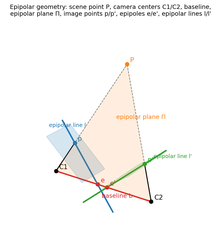
Epipolar geometry in one 3-D picture: scene point P, camera centers C1/C2 joined by the red baseline b, the orange epipolar plane Π through all three, the image points p/p′, the epipoles e/e′ where the baseline pierces the image planes, and the epipolar lines l/l′ where Π cuts the image planes. বাংলা: এক ছবিতে পুরো epipolar জ্যামিতি — scene point P, লাল baseline-এ যুক্ত দুই center C1/C2, তিনজনের কমলা epipolar plane Π, image point p/p′, baseline যেখানে image plane ফুটো করে সেই epipole e/e′, আর Π যেখানে ছবি দুটোকে কাটে সেই epipolar line l/l′।
Every definition of §2.4 is one labeled element here — this is the diagram to reproduce when the exam says "sketch the epipolar geometry". Note that both epipolar lines pass through their epipoles, and that rotating P around the baseline sweeps the whole pencil of epipolar planes.
বাংলা: পরীক্ষায় "epipolar geometry আঁকুন" এলে ঠিক এই ছবি: দুই center, baseline, P, plane, দুই লাইন, দুই epipole — সাতটা label। খেয়াল করুন: প্রতিটা epipolar line নিজের epipole দিয়ে গেছে, আর P-কে baseline-এর চারদিকে ঘোরালে plane-গুলোর গোটা পাখা (pencil) তৈরি হয়।
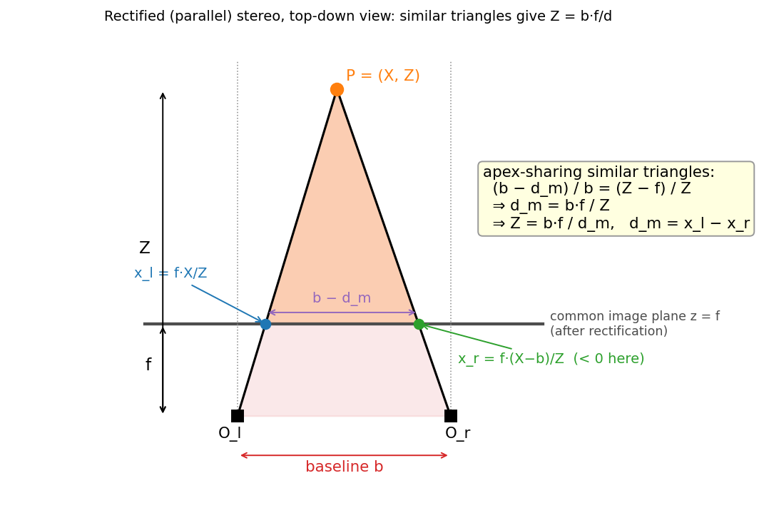
Top-down view of a rectified pair: camera centers O_l/O_r on the baseline b, the common image plane at z = f, scene point P = (X, Z), image points x_l = f·X/Z and x_r = f·(X−b)/Z, and the two shaded apex-sharing similar triangles whose ratio (b − d_m)/b = (Z − f)/Z yields Z = b·f/d. বাংলা: Rectified জোড়ার উপর-থেকে-দেখা: baseline b-তে দুই center, z = f-এ common image plane, scene point P, দুই image point — আর ছায়া দেওয়া দুই সদৃশ ত্রিভুজ, যাদের অনুপাত (b − d_m)/b = (Z − f)/Z থেকেই Z = b·f/d।
This is the picture behind the master formula — the stereo twin of Chapter 1's pinhole triangle figure. The yellow box on the right carries the full derivation chain; reproduce triangles + box and the derivation question is answered.
বাংলা: মূল সূত্রের জন্মস্থান এই ছবি — Chapter 1-এর pinhole ত্রিভুজেরই stereo সংস্করণ। দুই ত্রিভুজ আর হলুদ বাক্সের চার লাইন আঁকতে পারলেই derivation-প্রশ্নের পুরো নম্বর।
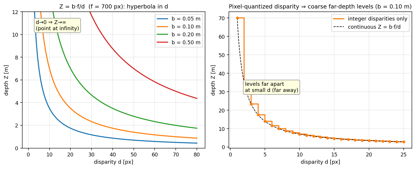
Left: Z = b·f/d (f = 700 px) for baselines 0.05–0.50 m — a hyperbola in d; d → 0 sends Z → ∞. Right: with integer disparities (b = 0.10 m) the measurable depths form a staircase Z_k = b·f/k whose steps grow huge at small d (far range). বাংলা: বাঁয়ে চারটি baseline-এর জন্য Z = b·f/d-এর অধিবৃত্ত — d → 0 মানেই Z → ∞। ডানে integer disparity-র সিঁড়ি: মাপা-সম্ভব depth-গুলো বিচ্ছিন্ন ধাপ Z_k = b·f/k, দূরে (ছোট d-তে) ধাপগুলো বিশাল ফাঁকা।
Two exam messages in one figure: disparity is inverse depth (hyperbola), and pixel quantization makes far depth coarse — the staircase is the discrete face of the ∂Z/∂d law. Larger baselines push the whole curve up: same disparity, more depth.
বাংলা: এক ছবিতে দুই বার্তা: disparity = উল্টানো depth (অধিবৃত্ত), আর pixel-quantization দূরের depth-কে মোটা দাগে মাপে (সিঁড়ি) — এটাই ∂Z/∂d সূত্রের চোখে-দেখা রূপ। Baseline বড় হলে গোটা curve উপরে ওঠে: একই disparity-তে বেশি depth।
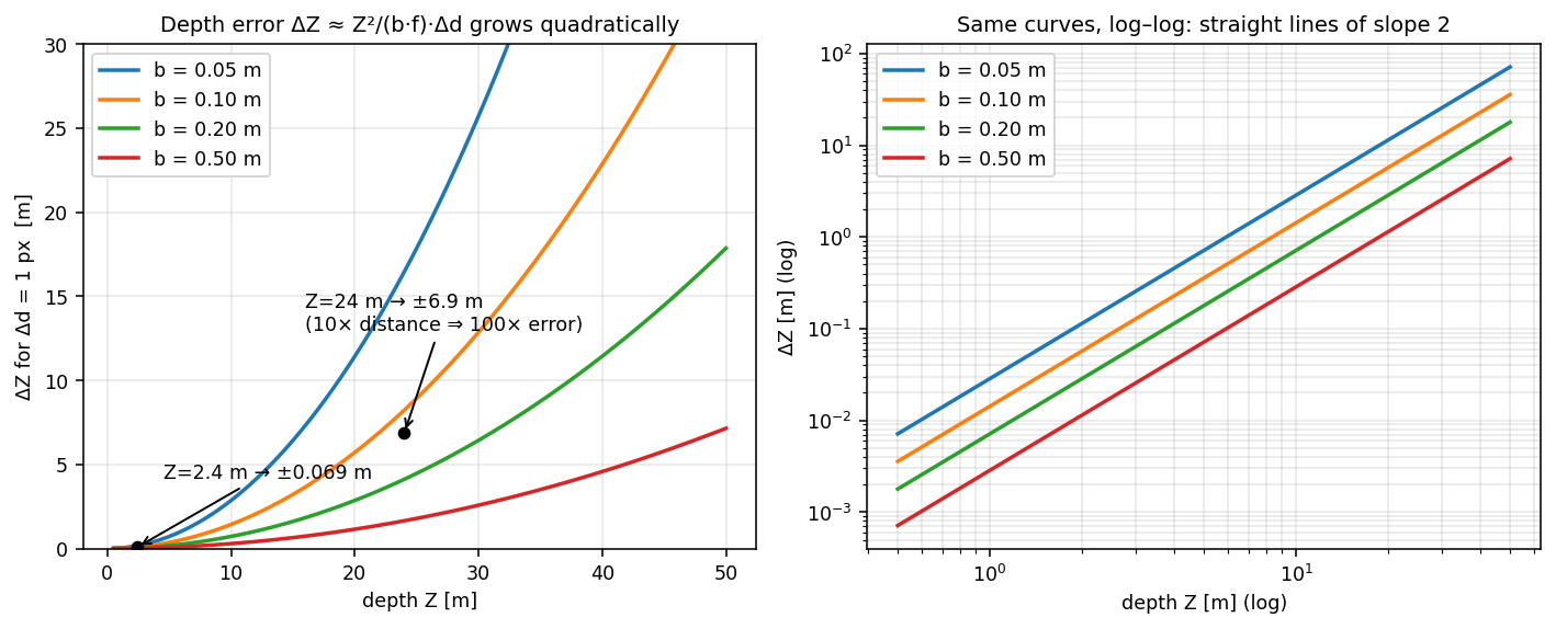
Depth uncertainty ΔZ ≈ Z²/(b·f)·Δd for Δd = 1 px and four baselines (f = 700 px). Left, linear axes: the b = 0.12-class curve passes ±0.069 m at Z = 2.4 m but ±6.9 m at Z = 24 m — 10× the distance, 100× the error. Right, log–log: all curves are straight lines of slope 2 — the visual signature of a quadratic law. বাংলা: ΔZ ≈ Z²/(b·f)·Δd — ১ pixel ভুলে depth-এর ভুল। বাঁয়ে সাধারণ অক্ষ: 2.4 m-এ ±৬.৯ cm, 24 m-এ ±৬.৯ m — দূরত্ব ১০ গুণ, ভুল ১০০ গুণ। ডানে log–log: সব রেখা ঢাল-২-এর সরলরেখা — বর্গ-নিয়মের সাক্ষর।
If an examiner asks "why do stereo cameras in cars only claim ~30 m useful range?", point here: with automotive baselines the error at large Z swallows the measurement. The log–log panel is the quickest proof that the exponent really is 2.
বাংলা: "গাড়ির stereo কেন ~৩০ মিটারের বেশি ভরসাযোগ্য নয়?" — উত্তর এই ছবি: দূরত্বের বর্গে ভুল বাড়ে, বড় Z-এ ভুলটা মাপকেই গিলে ফেলে। Log–log-এ ঢাল ২ — exponent যে সত্যিই ২, তার এক-নজরের প্রমাণ।
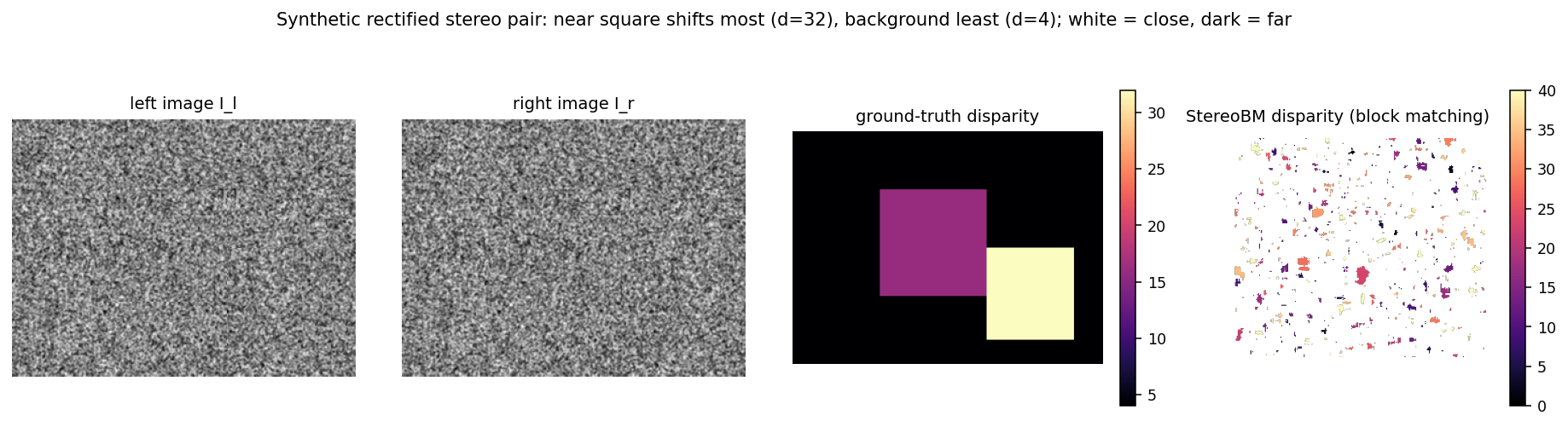
A synthetic rectified pair (textured background, two floating squares), the ground-truth disparity (background 4 px, middle square 16 px, near square 32 px) and the OpenCV StereoBM block-matching result (15×15 blocks, 48 disparities). Bright = near, dark = far. বাংলা: কৃত্রিম rectified জোড়া: texture-ভরা পটভূমি আর দুটি ভাসমান বর্গ; ground-truth disparity (পটভূমি ৪, মাঝের বর্গ ১৬, কাছের বর্গ ৩২ px) এবং StereoBM block-matching-এর ফল (১৫×১৫ window, ৪৮ disparity)। উজ্জ্বল = কাছে, অন্ধকার = দূরে।
Compare panels 3 and 4: the recovered map gets the three layers right, but the square boundaries are eroded/fattened by the window, and a vertical stripe at the left margin has no valid match (those pixels are only visible in one view — built-in occlusion). The textbook failure modes appear even in this perfectly clean synthetic scene.
বাংলা: ৩ আর ৪ নম্বর প্যানেল মিলিয়ে দেখুন: তিনটা স্তর ঠিকই ধরা পড়েছে, কিন্তু বর্গের কিনারাগুলো window-এর কারণে ক্ষয়ে/ফুলে গেছে, আর বাঁ প্রান্তের ফালিতে match নেই-ই (ওই pixel-গুলো এক ছবিতেই দৃশ্যমান — জন্মগত occlusion)। একদম পরিষ্কার কৃত্রিম দৃশ্যেও পাঠ্যবইয়ের ব্যর্থতাগুলো হাজির।
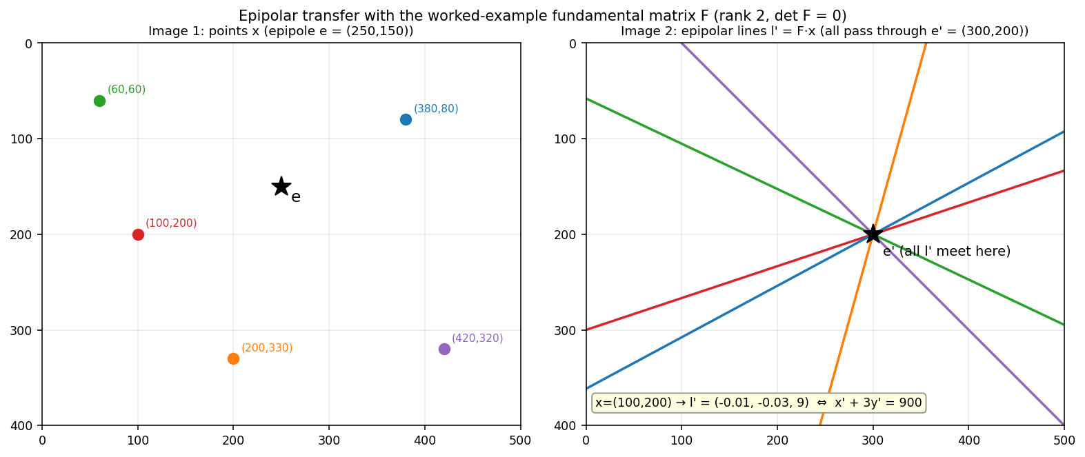
Five points in image 1 (left) and their epipolar lines l′ = F·x in image 2 (right), computed with the worked-example fundamental matrix of §4.8. All five lines intersect in the epipole e′ = (300, 200) — the null vector of Fᵀ; the epipole of image 1 sits at e = (250, 150). The yellow box spells out the §4.8 example: x = (100, 200) → x′ + 3y′ = 900. বাংলা: Image 1-এর পাঁচটি বিন্দু আর image 2-তে তাদের epipolar line l′ = F·x (§4.8-এর F দিয়ে)। পাঁচটি লাইনই epipole e′ = (300, 200)-তে মিলেছে — Fᵀ-এর null vector; image 1-এর epipole e = (250, 150)। হলুদ বাক্সে §4.8-এর হিসাব: x = (100, 200) → x′ + 3y′ = 900।
The picture is the rank-2 property: a full-rank matrix could never force five different lines through one point. Use it to remember the algebra: point in → line out (\(F\cdot x\)), all lines out → one point (\(F^{T}e' = 0\)).
বাংলা: Rank-2 ধর্মের ছবি-প্রমাণ: full-rank matrix কখনোই পাঁচটা আলাদা লাইনকে এক বিন্দুতে জড়ো করতে পারত না। মনে রাখার সূত্র: বিন্দু ঢোকে → লাইন বেরোয় (\(F\cdot x\)); সব লাইন → এক বিন্দু (epipole, \(F^{T}e' = 0\))।
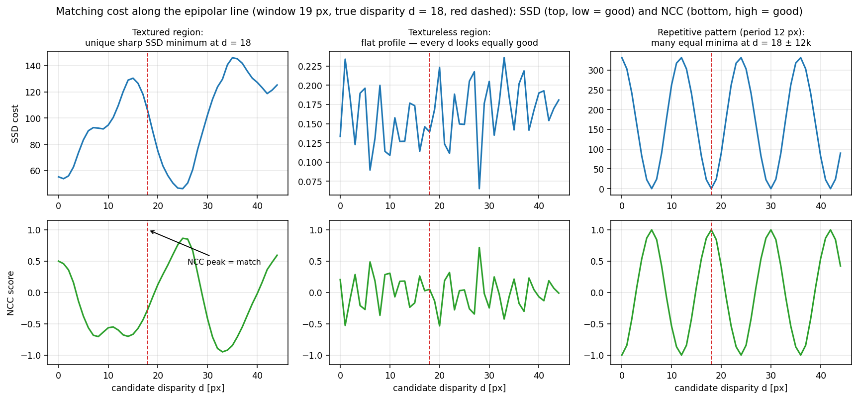
SSD cost (top, low = good) and NCC score (bottom, high = good) along the epipolar line for a 19-px window; the true disparity d = 18 is the red dashed line. Textured region: one sharp minimum/peak at 18. Textureless region: flat profiles — every disparity looks equally good. Repetitive pattern (period 12 px): equally deep minima at 18 ± 12k. বাংলা: Epipolar line ধরে SSD (উপরে, কম = ভালো) আর NCC (নিচে, বেশি = ভালো), window ১৯ px, আসল disparity ১৮ (লাল ড্যাশ)। Texture-ভরা অঞ্চল: ১৮-তে একটাই ধারালো minimum/শিখর। Texture-হীন: রেখা সমতল — সব d সমান "ভালো"। পুনরাবৃত্ত (period ১২): ১৮ ± ১২k-তে সমান গভীর অনেক minimum।
This is §4.11's failure-mode catalogue as data. The middle column explains why a white wall defeats any window-based method, and the right column why winner-take-all on a fence picks a random tooth — only a smoothness prior can break those ties.
বাংলা: §4.11-এর ব্যর্থতা-তালিকা এখানে data হয়ে ফুটেছে: সাদা দেয়ালে cost-রেখা সমতল (কোনো window-পদ্ধতিই বাঁচাতে পারে না), আর বেড়ার মতো প্যাটার্নে winner-take-all এলোমেলো একটা দাঁত বেছে নেয় — টাই ভাঙতে পারে কেবল smoothness prior।
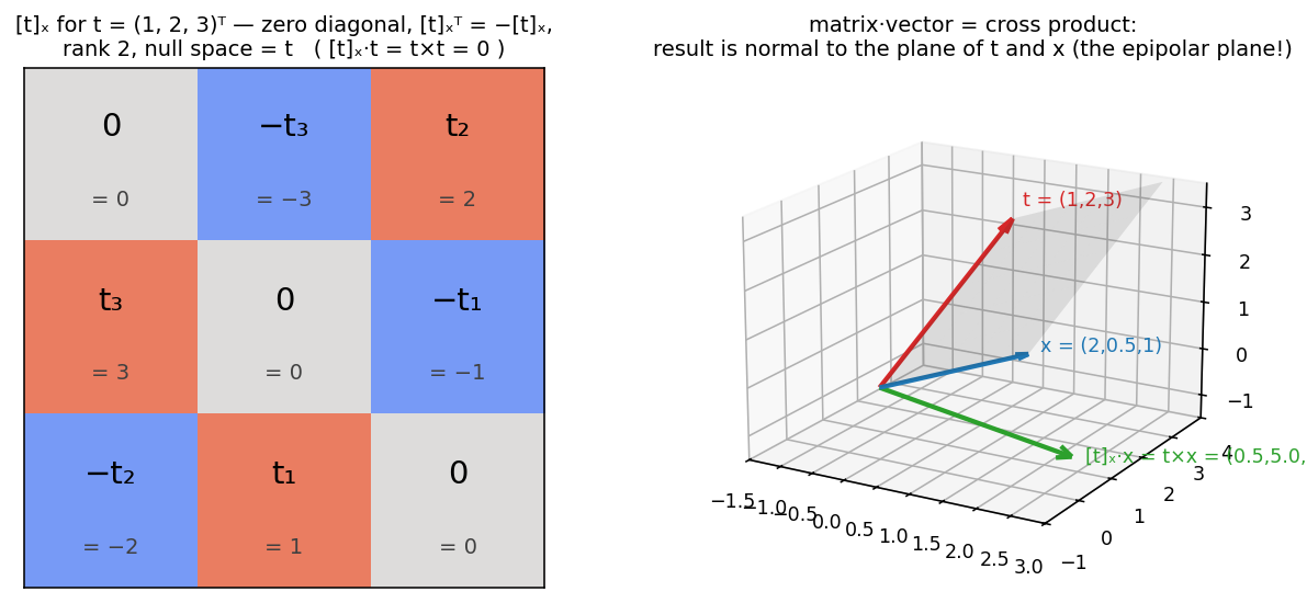
Left: the structure of [t]ₓ for t = (1, 2, 3)ᵀ — zero diagonal, mirrored signs ([t]ₓᵀ = −[t]ₓ), rank 2, null space = t itself. Right: matrix·vector = cross product — [t]ₓ·x = t × x is normal to the gray plane spanned by t and x; in the essential-matrix derivation that plane is the epipolar plane. বাংলা: বাঁয়ে t = (1, 2, 3)ᵀ-এর [t]ₓ-এর গঠন — কর্ণ শূন্য, আয়নায়-উল্টানো চিহ্ন, rank 2, null space = t। ডানে matrix-গুণ = cross product: [t]ₓ·x = t × x ফলটি t আর x-এর ধূসর সমতলের উপর লম্ব — E-এর derivation-এ ওই সমতলটাই epipolar plane।
Memorize the left panel's sign pattern (−t₃ top-middle is the anchor; the rest follows by antisymmetry). The right panel is the geometric heart of \(x'^{T}[t]_{x}Rx = 0\): the matrix output is the epipolar-plane normal, and the constraint says x′ is perpendicular to it.
বাংলা: বাঁ প্যানেলের চিহ্ন-নকশা মুখস্থ করুন (উপরের-মাঝে −t₃ ধরলেই বাকিটা antisymmetry-তে চলে আসে)। ডান প্যানেলই \(x'^{T}[t]_{x}Rx = 0\)-এর জ্যামিতিক হৃদয়: matrix-এর ফল epipolar plane-এর normal, আর শর্তটা বলে x′ সেই normal-এর উপর লম্ব — অর্থাৎ plane-এর ভেতরে।
§6 Algorithms & Code¶
6.1 The stereo block-matching pipeline (pseudocode)¶
rectify L, R                                  # epipolar lines → image rows
for each row y:
    for each pixel x in L:
        for each candidate disparity d in [d_min, d_max]:
            cost(d) = SAD( window_L(x, y), window_R(x − d, y) )
        disparity[y, x] = argmin_d cost(d)    # winner-take-all
optional: left-right consistency check → occlusion mask
optional: global smoothing (DP per scanline / graph cuts on the 2-D grid)
depth[y, x] = b · f_px / disparity[y, x]      # only if metric depth is needed
বাংলা: তিনটে nested loop — সারি, pixel, প্রার্থী disparity; প্রতি pixel-এ সবচেয়ে কম cost জেতে। তারপর ইচ্ছেমতো তিনটে polish: consistency check (occlusion ধরা), global smoothing (streak/noise কমানো), আর শেষে দরকার হলে \(Z = b\cdot f/d\)।
6.2 The 8-point algorithm (pseudocode)¶
normalize points per image: centroid → (0,0), RMS distance → √2   (T, T′)
for each correspondence (x, y) ↔ (x′, y′):
    add row [x′x, x′y, x′, y′x, y′y, y′, x, y, 1] to A
U, Σ, Vᵀ = SVD(A)
f = last column of V; F̂ = reshape(f, 3, 3)
U_F, (σ₁, σ₂, σ₃), V_Fᵀ = SVD(F̂);  F̂ = U_F·diag(σ₁, σ₂, 0)·V_Fᵀ   # enforce rank 2
F = T′ᵀ · F̂ · T                                                    # denormalize
বাংলা: মন্ত্র: normalize → A বানাও → SVD-র শেষ কলাম → rank-2 জোর করো → denormalize। বাস্তবে চারপাশে RANSAC জড়িয়ে outlier match ছেঁকে নেওয়া হয়।
6.3 Trial-exam Q7b in twelve lines of Python¶
import numpy as np

b   = 5.0            # baseline [cm]
f_cm = 5.0           # focal length [cm]
m   = 1.0            # pixel density [px/cm]  (from FOV 90°, 10 px over 10 cm)
f_px = m * f_cm      # = 5 px
o_x, o_y = 4.5, 5.0  # principal point [px]

def stereo_to_3d(xL, yL, xR):
    d = xL - xR                      # disparity [px]
    Z = b * f_px / d                 # depth [cm]
    X = (xL - o_x) * Z / f_px
    Y = (yL - o_y) * Z / f_px
    return np.array([X, Y, Z]), d

p1, d1 = stereo_to_3d(8, 5, 3)       # → [3.5, 0, 5.0],  d = 5
p2, d2 = stereo_to_3d(5, 5, 3)       # → [1.25, 0, 12.5], d = 2
print(p1, d1, p2, d2, p2 - p1)       # Δ = [-2.25, 0, 7.5]
The function is the whole of §4.3: disparity, then Z, then back-projected X, Y. Run it once before the exam and check the three printed results against §4.3.
বাংলা: §4.3-এর পাঁচটা ধাপ একটা function-এ: disparity → Z → X, Y। পরীক্ষার আগের রাতে একবার চালিয়ে §4.3-এর সংখ্যাগুলো মিলিয়ে নিন — [3.5, 0, 5], [1.25, 0, 12.5], \(\Delta = [-2.25, 0, 7.5]\)।
6.4 Block matching from scratch (SAD, winner-take-all)¶
import cv2, numpy as np

def block_match(L, R, max_d=64, win=5):
    H, W = L.shape
    pad = win // 2
    Lp = cv2.copyMakeBorder(L, pad, pad, pad, pad, cv2.BORDER_REFLECT)
    Rp = cv2.copyMakeBorder(R, pad, pad, pad, pad, cv2.BORDER_REFLECT)
    disp = np.zeros_like(L, dtype=np.int32)
    for y in range(H):
        for x in range(W):
            wL = Lp[y:y + win, x:x + win].astype(np.int32)
            best, best_d = np.inf, 0
            for d in range(min(x, max_d) + 1):          # search to the LEFT in R
                wR = Rp[y:y + win, x - d:x - d + win].astype(np.int32)
                cost = np.abs(wL - wR).sum()            # SAD
                if cost < best:
                    best, best_d = cost, d
            disp[y, x] = best_d
    return disp
Note the two conventions baked in: candidates are taken at \(x - d\) in the right image (a point moves left when the camera moves right), and \(\min (x, \max _{d})\) stops the window from running off the image — the built-in occlusion zone at the left border.
বাংলা: দুটো convention খেয়াল করুন: ডান ছবিতে প্রার্থী নেওয়া হয় \(x - d\)-তে (ক্যামেরা ডানে সরলে বিন্দু ছবিতে বাঁয়ে সরে), আর \(\min (x, \max _{d})\) বাঁ-কিনারার occlusion অঞ্চলে window-কে ছবির বাইরে যেতে দেয় না। np.abs(...).sum()-কে বর্গে বদলালেই SSD।
6.5 Production route: OpenCV StereoSGBM + depth conversion¶
import cv2, numpy as np
imgL = cv2.imread('left.png',  cv2.IMREAD_GRAYSCALE)   # must be rectified!
imgR = cv2.imread('right.png', cv2.IMREAD_GRAYSCALE)

stereo = cv2.StereoSGBM_create(minDisparity=0, numDisparities=64,
                               blockSize=5, P1=8 * 5**2, P2=32 * 5**2)
disp = stereo.compute(imgL, imgR).astype(np.float32) / 16.0   # SGBM scales by 16

b, f_px = 0.05, 500                                    # 5 cm baseline, 500 px focal
Z = (b * f_px) / np.maximum(disp, 1e-3)                # guard against d ≤ 0
\(P1/P2\) are exactly the smoothness penalties of §2.10 (small/large disparity jumps); numDisparities must be a multiple of 16; the \(/16\) undoes OpenCV's fixed-point encoding — forgetting it scales all depths by 16.
বাংলা: \(P1/P2\) হলো §2.10-এর smoothness জরিমানা; numDisparities ১৬-এর গুণিতক হতে হয়; আর \(/16.0\) ভুললে সব depth ১৬ গুণ ভুল — OpenCV disparity-কে fixed-point-এ ১৬ গুণ করে রাখে। np.maximum(disp, 1e-3) হলো \(d \to 0\)-তে \(Z \to \infty\) বিস্ফোরণের বিমা।
6.6 Fundamental matrix with RANSAC + drawing epipolar lines¶
import cv2, numpy as np
F, mask = cv2.findFundamentalMat(pts1, pts2, cv2.FM_RANSAC, 3.0)
pts1_in, pts2_in = pts1[mask.ravel() == 1], pts2[mask.ravel() == 1]

def draw_epilines(img, lines, pts):
    out = img.copy(); h, w = img.shape[:2]
    for l, p in zip(lines, pts):
        a, b, c = l.ravel()                       # line a·x + b·y + c = 0
        x0, y0 = 0, int(round(-c / b))            # intersection with x = 0
        x1, y1 = w, int(round(-(c + a * w) / b))  # intersection with x = w
        cv2.line(out, (x0, y0), (x1, y1), (0, 255, 0), 1)
        cv2.circle(out, tuple(map(int, p)), 4, (0, 0, 255), -1)
    return out

lines2 = cv2.computeCorrespondEpilines(pts1_in, 1, F).reshape(-1, 3)  # l′ = F·x
img2_out = draw_epilines(img2, lines2, pts2_in)
The drawing trick: a line (a, b, c) is rendered by computing its y at the left edge (\(x = 0\)) and the right edge (\(x = w\)). Each drawn circle (the matched point) should sit on its line — the visual version of \(u'^{T}Fu = 0\).
বাংলা: লাইন (a, b, c) আঁকার কৌশল: বাঁ প্রান্তে (\(x = 0\)) আর ডান প্রান্তে (\(x = w\)) y-মান বের করে দুই বিন্দু জুড়ে দেওয়া। প্রতিটা লাল বিন্দু (match) নিজের সবুজ লাইনের উপর বসা উচিত — \(u'^{T}Fu = 0\)-এর চোখে-দেখা প্রমাণ; না বসলে সেটা RANSAC-এর ফেলে দেওয়া outlier।
6.7 Census transform + Hamming distance¶
import numpy as np

def census(img, win=3):
    H, W = img.shape
    pad = win // 2
    out = np.zeros((H, W), np.uint64)
    for dy in range(-pad, pad + 1):
        for dx in range(-pad, pad + 1):
            if dx == 0 and dy == 0:
                continue
            shifted = np.roll(img, (dy, dx), (0, 1))
            out = (out << 1) | (shifted < img)      # bit = "neighbor darker than me?"
    return out

def hamming(a, b):
    x = np.bitwise_xor(a, b)                        # differing bits
    return np.unpackbits(x.view(np.uint8).reshape(-1, 8),
                         axis=1).sum(axis=1).reshape(a.shape)
Each pixel becomes an 8-bit signature of orderings, not intensities — any monotonic lighting change (gamma, exposure, contrast) leaves every "brighter than?" answer unchanged, so the census cost is unaffected where SAD/SSD collapse.
বাংলা: প্রতিটা pixel হয়ে যায় ৮-বিটের স্বাক্ষর — মান নয়, ক্রম: প্রতিবেশী আমার চেয়ে অন্ধকার কি না। আলোর যেকোনো monotonic বদলে (exposure, gamma, contrast) এই হ্যাঁ/না উত্তরগুলো বদলায় না — তাই census + Hamming টেকে, যেখানে SAD/SSD ভেঙে পড়ে।
6.8 The 8-point algorithm from scratch (with Hartley normalization)¶
import numpy as np

def normalize(pts):                                  # pts: (n, 2)
    c = pts.mean(axis=0)
    rms = np.sqrt(((pts - c) ** 2).sum(axis=1).mean())
    s = np.sqrt(2) / rms
    T = np.array([[s, 0, -s * c[0]], [0, s, -s * c[1]], [0, 0, 1]])
    ph = np.column_stack([pts, np.ones(len(pts))])
    return (T @ ph.T).T, T

def eight_point(p1, p2):
    n1, T1 = normalize(p1)
    n2, T2 = normalize(p2)
    A = np.column_stack([n2[:, 0] * n1[:, 0], n2[:, 0] * n1[:, 1], n2[:, 0],
                         n2[:, 1] * n1[:, 0], n2[:, 1] * n1[:, 1], n2[:, 1],
                         n1[:, 0], n1[:, 1], np.ones(len(p1))])
    _, _, Vt = np.linalg.svd(A)
    F = Vt[-1].reshape(3, 3)                         # smallest-σ right vector
    U, S, Vt = np.linalg.svd(F)
    F = U @ np.diag([S[0], S[1], 0]) @ Vt            # enforce rank 2
    F = T2.T @ F @ T1                                # denormalize
    return F / F[2, 2]                               # fix the free scale
Every line maps to a step of §4.9; comment out normalize once on real pixel data and watch the epipolar lines fly off the image — the cheapest possible demonstration of conditioning.
বাংলা: §4.9-এর প্রতিটা ধাপ এখানে এক-এক লাইনে। একবার পরীক্ষা করে দেখুন: normalize বাদ দিয়ে আসল pixel data-তে চালালে epipolar line-গুলো ছবির বাইরে উড়ে যায় — ill-conditioning-এর সবচেয়ে সস্তা হাতে-কলমে প্রমাণ।
6.9 Exercise Sheet 6 — the course code files explained¶
Ex/6/sheet6/epipolar_geometry.py — the geometry half of the sheet:
1. Loads an image pair, runs SIFT, matches descriptors with the ratio test → sparse correspondences (Chapter 5 machinery).
2. Estimates F with cv2.findFundamentalMat(..., FM_RANSAC) — RANSAC discards mismatches that would poison the linear system.
3. Draws epipolar lines: for chosen points in image 1 it computes \(l' = F\cdot x\) and renders them in image 2 (and back with \(F^{T}\) — those lines all pass through the original point's epipolar line pencil).
4. Calls cv2.stereoRectifyUncalibrated to get the homographies \(H_{1}, H_{2}\) and warps both images so the epipolar lines become horizontal.
Ex/6/sheet6/stereo_depth.py — the depth half, on already-rectified images:
* For each pixel, a scanline search compares summed-RGB descriptors within a disparity range (with care at the image borders), takes the best match, computes \(d = x_{l} - x_{r}\), and converts to relative depth via \(Z \propto 1/d\). It is exactly §6.4 with a color cost — and exhibits exactly the §4.11 failure modes on textureless areas.
Ex/6/sheet6/pt_depth.py — monocular depth in ~20 lines:
* Pulls a pretrained MiDaS / ZoeDepth model from torch.hub, applies the model's own resize/normalize transforms, runs one forward pass, and visualizes the predicted inverse-depth map with a colormap. Confirms §2.12: gorgeous relative depth, no metric scale.
Ex/6/sheet6/depth_utils.py — shared helpers: normalizing depth maps to [0, 1], applying colormaps, saving point clouds for 3-D viewing.
বাংলা: Sheet 6-এর চার ফাইলের শ্রম-বিভাজন: epipolar_geometry.py = জ্যামিতি (SIFT match → RANSAC-এ F → epipolar line আঁকা → uncalibrated rectification); stereo_depth.py = গভীরতা (rectified ছবিতে scanline খোঁজ, RGB-যোগফল cost, \(d = x_{l} - x_{r}\), \(Z \propto 1/d\)); pt_depth.py = এক-ছবির depth (torch.hub থেকে MiDaS নামিয়ে inverse-depth আঁকা — আপেক্ষিক depth, metric নয়); depth_utils.py = সাহায্যকারী (normalize, colormap, point cloud)। পরীক্ষায় "code কী করত" ধাঁচের প্রশ্নে এই চার-লাইনের সারাংশই যথেষ্ট।
§7 Trial-Exam Mapping¶
| Trial-exam item | What you must know | Where in this chapter |
|---|---|---|
| Q7a — describe how to compute depth from a stereo pair with given correspondences | Rectify → disparity \(d = x_{l} - x_{r}\) → \(Z = b\cdot f_{px}/d\) → back-project X, Y; mention unit handling |
§2.3, §4.2, §4.3 |
| Q7b-i — 3-D positions of two correspondences | Pixel density from FOV (1 px/cm), \(Z = b\cdot f/d\), \(X = (x_{l} - o_{x})\cdot Z/f\), \(Y = (y_{l} - o_{y})\cdot Z/f\) → (3.5, 0, 5) and (1.25, 0, 12.5) cm | §4.3 worked example, §6.3 |
| Q7b-ii — ΔX, ΔY, ΔZ between them | Simple subtraction: (−2.25, 0, 7.5) cm | §4.3 step 4 |
| Q7b-iii — disparities of both points | \(d_{1} = 8 - 3 = 5 px\), \(d_{2} = 5 - 3 = 2 px\); larger disparity = closer point | §4.3 step 1 |
| Q7c — briefly describe optical axis and epipolar line | Two crisp definitions, see model answers below | §2.4, §4.1 |
Model answer (Q7a): "Rectify both images so that epipolar lines coincide with image rows. For each given correspondence compute the disparity d = x_l − x_r. With baseline b and focal length f (converted to pixel units via the pixel density), the depth is Z = b·f/d; the remaining coordinates follow by back-projection, X = (x_l − o_x)·Z/f and Y = (y_l − o_y)·Z/f."
Model answer (Q7c — optical axis): "The optical axis is the line through the camera center (lens center) perpendicular to the image plane; it meets the image at the principal point and gives the camera's viewing direction."
Model answer (Q7c — epipolar line): "For a point in one image, the epipolar line is the line in the other image on which the corresponding point must lie; it is the projection of the first camera's viewing ray into the second image — equivalently, the intersection of the epipolar plane with the second image plane. In a rectified pair the epipolar lines are the horizontal scanlines."
বাংলা: Q7-এর দশ নম্বরের পুরোটা এই chapter-এ: পদ্ধতির বর্ণনা (§4.2–§4.3-এর রেসিপি), সংখ্যার হিসাব (§4.3-এর worked example হুবহু), আর দুটো সংজ্ঞা (উপরের model answer দুটি প্রায় মুখস্থ-মানের করে রাখুন)। সময় বাঁচাতে: আগে disparity দুটো লিখুন (৫ আর ২), তারপর Z, তারপর X-Y — আর শেষ লাইনে এক-বাক্যের sanity check।
§8 Mock Exam — 20 Questions¶
Answer everything on paper first; full worked solutions follow in §8.5. Tier A = basics, B = intuition, C = harder computation/derivation, D = transfer questions slightly beyond the lecture (typical for a tough oral or a "Transfer" section in the written exam).
Tier A — Basic (definitions & direct formula use)¶
A1. Define baseline, epipolar plane, epipolar line, and epipole. Then explain in one sentence why every epipolar line of an image must pass through that image's epipole.
A2. A rectified stereo rig has baseline \(b = 0.1 m\) and focal length \(f = 700 px\). A feature is matched with disparity \(d = 14 px\). Compute the depth Z. What happens to Z as \(d \to 0\), and which scene points have \(d = 0\)?
A3. In a rectified pair, two correspondences are given as \((x_{l}, y_{l}) \leftrightarrow (x_{r}, y_{r})\): point 1 = (60, 50) ↔ (50, 50), point 2 = (80, 50) ↔ (65, 50). With \(b = 0.05 m\) and \(f = 500 px\), compute both disparities and both depths. Which point is closer, and how could you have known before computing the depths?
A4. Write down the epipolar constraint using the fundamental matrix. State the size, rank, and number of degrees of freedom of F, and say in words what \(l' = F\cdot x\) is.
A5. What two geometric properties hold after stereo rectification? Write down the rectified fundamental matrix F*, show which scalar constraint \(x'^{T}F*x = 0\) reduces to, and state where the epipoles lie after rectification.
Tier B — Intuitive (why / when)¶
B6. Why is depth fundamentally unrecoverable from a single (uncalibrated, unfamiliar) image? Explain how the Ames-room illusion exploits this — and why the illusion would collapse immediately for a stereo camera.
B7. Hold a finger 20 cm in front of your face and alternately close the left and right eye: the finger jumps, the far wall barely moves, and the moon outside the window does not move at all. Explain all three observations with one formula, and connect the moon case to the epipoles of a rectified (parallel) camera pair.
B8. Describe the window-size dilemma of block matching: what goes wrong with too-small windows, what with too-large windows? Name the artifact that large windows cause at depth boundaries, and explain why no single window size can be correct everywhere.
B9. You may build your stereo rig with a 5 cm or a 50 cm baseline. Using \(|\Delta Z| \approx Z^{2}/(b\cdot f)\cdot \Delta d\), explain what the long baseline buys you — and list two things it costs you on the matching side. Why do phone "portrait mode" rigs nevertheless use tiny baselines?
B10. Write down the left-right consistency check and explain (a) why an occluded pixel fails it, and (b) why a correctly matched pixel passes it. What does a stereo system typically do with pixels that fail?
Tier C — Harder (multi-step computation / derivation)¶
C11. A camera has focal length \(f = 4 mm\) and square pixels of size \(2 \mu m\); the stereo baseline is \(b = 0.12 m\). A point is matched with disparity \(d = 60 px\). (a) Convert the focal length to pixels. (b) Compute the depth Z — show the units cancelling. © Compute the depth uncertainty for a matching error of \(\Delta d = 1 px\), in two ways: via \(b\cdot f/d^{2}\) and via \(Z^{2}/(b\cdot f)\).
C12. Use the fundamental matrix of §4.8:
For the point \(x = (50, 100)\) in image 1, compute the epipolar line \(l' = F\cdot x\), scale it to integer coefficients, and verify that the epipole \(e' = (300, 200)\) lies on it. Then decide which of the candidates (100, 150) and (200, 150) is geometrically admissible as the match.
C13. (Design problem.) You must configure a block matcher for a rig with \(b = 0.1 m\), \(f = 500 px\) that should measure depths from 1 m to 4 m. (a) Compute the disparity range that the search must cover. (b) You use an OpenCV-style matcher whose numDisparities must be a multiple of 16; propose minDisparity and numDisparities. © Compute the depth quantization step (Δd = 1 px) at both ends of the range — is the precision requirement "±5 cm at 4 m" achievable without sub-pixel refinement?
C14. (Triangulation, numeric.) A rectified rig has \(b = 0.2 m\), \(f = 500 px\), principal point \((o_{x}, o_{y}) = (320, 240)\). A point is observed at (420, 290) in the left image and (370, 290) in the right image. Compute its full 3-D position (X, Y, Z) in the left-camera frame. What would it tell you if the two y-coordinates had differed?
C15. Re-solve the complete trial-exam Q7b from scratch without looking at §4.3: cameras rectified and parallel, \(b = 5 cm\), \(f = 5 cm\), FOV 90°, image 10×10 px, principal point (4.5, 5); correspondences (8, 5) ↔ (3, 5) and (5, 5) ↔ (3, 5). Compute the pixel density, both disparities, both 3-D positions, and \((\Delta X, \Delta Y, \Delta Z)\). Then check yourself against §4.3.
Tier D — Transfer (adjacent to, but beyond, the lecture)¶
D16. E and F both have rank 2 — yet E has 5 DOF and F has 7. (a) Derive both counts. (b) State the extra algebraic property that distinguishes a valid essential matrix from a generic rank-2 matrix (think singular values), and sketch why it holds for \(E = [t]_{x}R\). © Give the minimal number of correspondences for estimating F and for estimating E, and explain where the difference comes from.
D17. Identify and analyze two degenerate configurations for two-view geometry: (a) the camera purely rotates between the two shots (zero baseline) — what is E, what happens to depth recovery, and which 3×3 entity correctly relates the two images instead? (b) All visible scene points lie on a single plane — show why \(x'^{T}Fx = 0\) no longer determines F uniquely, and name the practical consequence for the 8-point algorithm.
D18. (Active stereo / structured light.) A depth sensor projects a known infrared dot pattern onto the scene and observes it with one camera (e.g., Kinect v1). (a) Which fundamental failure mode of passive stereo does the projected pattern eliminate, and why? (b) Explain in what sense the projector acts as the "second camera" of a stereo pair. © Why does this technology degrade in bright sunlight, and what does that imply about indoor vs outdoor use?
D19. (Time-of-flight vs stereo.) A ToF camera measures depth from the round-trip time of emitted light, with a roughly distance-independent error of a few centimeters. Compare ToF and passive stereo on: error growth with distance, textureless surfaces, operation in darkness, spatial resolution, and characteristic artifacts. Which would you choose for (i) a robot navigating a dark warehouse, and (ii) long-range automotive perception — and why?
D20. (Numerics of the 8-point algorithm.) Correspondences live around \((x, y) \approx (1000, 500)\) in both images. (a) Estimate the magnitudes of the nine entries of one row of the matrix A and the spread between the largest and smallest. (b) Explain why this spread poisons precisely the quantity the algorithm needs (the smallest-singular-value vector), in terms of the conditioning of A. © State Hartley's normalization precisely, and what the row entries look like afterwards. (d) Why must the resulting F̂ be denormalized, and how?
§8.5 Solutions¶
Tier A¶
A1.
Baseline: the line segment connecting the two camera centers \(C, C'\) (length b). Epipolar plane: the plane spanned by \(C, C'\) and the scene point P — one per scene point, all containing the baseline. Epipolar line: the intersection of the epipolar plane with an image plane; epipolar lines come in corresponding pairs. Epipole: the point where the baseline (extended) pierces the image plane — equivalently the image of the other camera's center.
Why all epipolar lines pass through the epipole: every epipolar plane contains the baseline, so every intersection of such a plane with the image plane contains the point where the baseline pierces that image plane — the epipole.
বাংলা: চারটে সংজ্ঞাই "C, C′, P" ছবিটা থেকে পড়া যায়; আর সব epipolar plane-এর ভেতরে baseline থাকে বলেই তাদের সব ছেদরেখা epipole দিয়ে যায় — এক লাইনের যুক্তি, মুখস্থ রাখুন।
A2.
As \(d \to 0\), \(Z = b\cdot f/d \to \infty\): the formula blows up because zero disparity means the two viewing rays are parallel. Points at infinity (in practice: extremely distant points like the moon, stars, far mountains) have \(d = 0\) — they appear at the same pixel in both views. বাংলা: \(Z = 70/14 = 5 m\)। \(d \to 0\) মানে দুই ray সমান্তরাল — বিন্দুটা অসীমে; চাঁদ-তারা দুই ছবিতে একই জায়গায় পড়ে, তাই stereo তাদের দূরত্ব মাপতে পারে না।
A3.
Point 2 is closer. Known in advance because it has the larger disparity — disparity is inverse depth, so the bigger jump between the views always belongs to the nearer point. বাংলা: disparity ১০ বনাম ১৫ — বড় disparity মানেই কাছের বিন্দু, depth না কষেই বলা যায়; হিসাবও তাই বলল: 2.5 m বনাম 1.67 m।
A4.
F is 3×3, has rank 2, and 7 degrees of freedom (9 entries − 1 for overall scale − 1 for the constraint \(\det F = 0\)). \(l' = F\cdot x\) is the epipolar line of x in the second image: the line on which the correspondence of x must lie; its three components are the line coefficients (a, b, c) of \(a\cdot x' + b\cdot y' + c = 0\).
বাংলা: এক সমীকরণ + তিন তথ্য: \(x'^{T}Fx = 0\); 3×3, rank 2, DOF 7 (scale −1, det = 0 −1)। \(F\cdot x\) মানে বিন্দু ঢুকল, অন্য ছবির লাইন বেরোলো — match সেই লাইনেই।
A5. After rectification: (i) both images lie in a common image plane whose normal is perpendicular to the baseline (cameras "look parallel"), and (ii) corresponding epipolar lines coincide with the same image row, so correspondence search is 1-D along scanlines.
(Expanding: \((x', y', 1)\cdot F*\cdot (x, y, 1)^{T} = (x',y',1)\cdot (0, -1, y)^{T} = -y' + y\).) The epipoles move to infinity in the direction of the baseline, \(e \simeq (\pm 1, 0, 0)^{T}\) — the baseline never pierces the (now parallel) image planes. বাংলা: Rectification-এর দুই উপহার: এক image plane, আর "match একই row-তে" (\(y' = y\))। F* মুখস্থ — মাঝে −1/1-এর ঘূর্ণি, বাকি শূন্য; epipole চলে যায় অসীমে \((\pm 1, 0, 0)^{T}\)।
Tier B¶
B6. A camera maps the whole viewing ray \({C + s\cdot r}\) to one pixel — depth along the ray is annihilated. From one image, a small-near object and a large-far object are identical stimuli, so depth is unrecoverable without prior knowledge. The Ames room is built distorted (sloping floor, trapezoidal walls) so that from one specific peephole its projection equals that of a normal rectangular room; the brain picks the familiar interpretation and concludes the two people must differ wildly in size. A stereo camera takes two views: the distorted room produces parallax that does not match a rectangular room's parallax — the disparities directly reveal the true geometry, and the illusion dies. বাংলা: এক ছবি = এক ray-এর সব বিন্দু এক pixel-এ — depth মুছে যায়; Ames room ঠিক এই ফাঁকটাই ব্যবহার করে এক peephole থেকে। দ্বিতীয় viewpoint এলেই parallax আসল জ্যামিতি ফাঁস করে দেয়।
B7.
The formula is \(d = b\cdot f/Z\). The finger: tiny Z (0.2 m) ⇒ huge disparity ⇒ big jump. The wall: larger Z ⇒ disparity shrinks proportionally to \(1/Z\). The moon: \(Z \approx 3.8\cdot 10^{8} m\) ⇒ \(d \approx 0\) to far below a pixel — the moon lands on the same image position in both views, which is why it seems to "follow" a moving car (no parallax = perceived as attached to you). Connection to epipoles: for parallel cameras the epipoles sit at infinity in the baseline direction, and a point at infinity projects to the same pixel in both images — \(d = 0\) is the statement that infinitely distant points coincide with their own correspondence.
বাংলা: সব এক সূত্রে: \(d = b\cdot f/Z\) — আঙুল (ছোট Z) লাফায়, দেয়াল কম, চাঁদ (\(Z \approx 3.8\times 10^{8} m\)) একদমই না; parallax শূন্য বলেই চাঁদ "পিছু নেয়"। Parallel ক্যামেরায় epipole অসীমে — অসীমের বিন্দুর disparity 0, দুটো একই কথা।
B8. Too small: the window contains too little structure — the cost is dominated by noise, and in homogeneous regions the profile is flat, so the argmin is random (the matcher is "blind"). Too large: the window straddles surfaces at different depths; the fronto-parallel assumption (one disparity for the whole window) breaks on slanted surfaces, and at object boundaries the strong foreground texture wins votes for background pixels too — the foreground fattening artifact (objects grow a halo of wrong depth). No single size works because the right size depends on local texture density and local depth variation, which change across the image — the motivation for adaptive windows and global methods. বাংলা: ছোট window = তথ্য কম, noise-এর হাতে সিদ্ধান্ত; বড় window = এক window-তে দুই depth ঢুকে পড়ে — কিনারায় "foreground fattening" (বস্তু মোটা হয়ে যায়)। সঠিক মাপ জায়গাভেদে আলাদা বলে এক মাপ কোথাও নেই — তাই global method।
B9.
The error law \(|\Delta Z| \approx Z^{2}/(b\cdot f)\cdot \Delta d\) has b in the denominator: a 10× longer baseline gives 10× finer depth at the same range (or the same precision √10× farther). Costs of the long baseline: (1) the two views differ much more (strong perspective/appearance change), so window-based matching becomes harder and more ambiguous; (2) far more occlusion — many points visible in only one camera — and a reduced overlapping field of view, plus a larger minimum measurable distance. Phones use millimeter–centimeter baselines because their subjects are close (Z small keeps \(Z^{2}/(b\cdot f)\) tolerable), the device must stay pocketable, and portrait mode only needs relative foreground/background separation, not metric precision.
বাংলা: b হরে বসে আছে — baseline ১০ গুণ, ভুল ১০ ভাগের ১। কিন্তু দাম: দুই view-এর চেহারা বেশি আলাদা (matching কঠিন) আর occlusion বেশি। ফোনের subject কাছে থাকে বলে ছোট baseline-ই যথেষ্ট — দরকার তো শুধু সামনে-পেছনে আলাদা করা, মিটার-নিখুঁত depth নয়।
B10.
(Signs per the convention \(d_{LR} = x_{l} - x_{r} \ge 0\), \(d_{RL} = x_{r} - x_{l} \le 0\); a consistent pair sums to ≈ 0.)
(a) An occluded pixel is visible only in the left image; its "match" in the right image is actually the projection of some other (foreground) scene point. Matching that right pixel back lands on that other point's left-image position — not on (x, y) — so the round trip fails.
(b) For a correct match, L→R lands on the true correspondence and R→L returns exactly to the start (up to noise ≤ 1 px), so the two disparities cancel. Failed pixels are marked in an occlusion mask and either left empty or filled by inpainting/extrapolation from the background side — they are not given fake matches.
বাংলা: যাও-এসো পরীক্ষা: বাঁ→ডান গিয়ে ডান→বাঁ ফিরলে নিজের ঘরে ফেরা উচিত; occluded pixel-এর "match" আসলে অন্য বিন্দুর ছবি, তাই সে অন্য ঘরে ফেরে — ধরা পড়ে। ব্যর্থ pixel-কে জোর করে match দেওয়া হয় না, occlusion mask-এ আলাদা রাখা হয়।
Tier C¶
C11.
(a)  f_px = f / pixel size = 4·10⁻³ m / 2·10⁻⁶ m = 2000 px

(b)  Z = b·f_px/d = (0.12 m · 2000 px) / (60 px) = 240 m·px / 60 px = 4 m
     (px cancels against px; Z inherits the meters of b)

(c)  way 1:  |ΔZ| = b·f/d² · Δd = 240/60² = 240/3600 ≈ 0.067 m
     way 2:  |ΔZ| = Z²/(b·f) · Δd = 16/240        ≈ 0.067 m     ✓ identical
So this rig measures the 4 m point to about ±7 cm per pixel of matching error. বাংলা: আগে mm→px (\(4 mm / 2 \mu m = 2000 px\)), তারপর \(Z = 240/60 = 4 m\) — একক কাটাকাটি দেখিয়ে লিখুন। ভুলের দুই সূত্র একই উত্তর দেয় (≈ 6.7 cm/px) — পরীক্ষায় দুটোই লিখে ✓ মেলালে নম্বর নিরাপদ।
C12.
Epipole check: \(300 - 4\cdot 200 + 500 = 300 - 800 + 500 = 0\) ✓ (every epipolar line passes through \(e'\)).
Candidates: (100, 150): \(100 - 600 + 500 = 0\) ✓ admissible — it lies exactly on the line. (200, 150): \(200 - 600 + 500 = 100 \neq 0\) ✗ rejected: it violates the epipolar constraint, so it cannot be the match no matter how similar the pixels look.
বাংলা: তিনটে dot product-এই লাইন: \((0.01, -0.04, 5)\), সুন্দর রূপ \(x' - 4y' + 500 = 0\); epipole বসিয়ে 0 পাওয়া মানেই অঙ্ক ঠিক পথে। প্রার্থী যাচাই: লাইনে বসলে গ্রহণযোগ্য (100,150 ✓), না বসলে pixel না দেখেই বাতিল (200,150 ✗)।
C13.
(a)  d = b·f/Z,  b·f = 0.1·500 = 50 m·px
     Z = 1 m → d = 50 px        Z = 4 m → d = 12.5 px
     required search range: d ∈ [12.5, 50] px

(b)  minDisparity = 12;  span needed ≈ 50 − 12 = 38 → numDisparities = 48
     (multiple of 16; covers d ∈ [12, 60) — margin on both ends)

(c)  ΔZ = Z²/(b·f)·Δd:
     at Z = 1 m:  1/50  = 0.02 m  (±2 cm)
     at Z = 4 m:  16/50 = 0.32 m  (±32 cm)
The requirement "±5 cm at 4 m" is not achievable with integer disparities (step 0.32 m). Options: sub-pixel refinement to \(\Delta d \approx 0.05/0.32 \approx 0.16 px\) (aggressive but possible with parabola fitting), or redesign the rig: increase \(b\cdot f\) by the factor \(0.32/0.05 = 6.4\) (e.g., baseline 0.32 m and f = 1000 px).
বাংলা: নকশার ছক: আগে দুই প্রান্তের disparity (50 আর 12.5 px), তারপর ১৬-র গুণিতকে search-পরিসর (min 12, num 48), শেষে দুই প্রান্তের quantization ধাপ (২ cm বনাম ৩২ cm)। ৪ মিটারে ±৫ cm চাইলে হয় sub-pixel (~0.16 px) নয় \(b\cdot f\) ৬.৪ গুণ — integer pixel-এ অসম্ভব, এটা স্পষ্ট করে লিখুন।
C14.
d = 420 − 370 = 50 px
Z = b·f/d        = (0.2 · 500)/50    = 100/50 = 2 m
X = (x_l − o_x)·Z/f = (420 − 320)·2/500 = 100·2/500 = 0.4 m
Y = (y_l − o_y)·Z/f = (290 − 240)·2/500 =  50·2/500 = 0.2 m

P = (0.4, 0.2, 2.0) m   in the left-camera frame
If the y-coordinates had differed, the pair would violate the rectified epipolar constraint \(y' = y\) — meaning either the images are not properly rectified (calibration error) or the correspondence is simply a mismatch; in both cases the depth formulas must not be applied to it. বাংলা: রেসিপি অপরিবর্তিত: \(d = 50\), \(Z = 2 m\), তারপর principal point বাদ দিয়ে scale — \(P = (0.4, 0.2, 2.0) m\)। y দুটো আলাদা হলে হয় rectification ভুল, নয় match-টাই ভুল — তখন সূত্রে হাতই দেবেন না।
C15. Full chain (must reproduce §4.3):
pixel density:  FOV 90° ⇒ half-width = f·tan 45° = 5 cm ⇒ width 10 cm / 10 px ⇒ m = 1 px/cm
                f_px = m·f = 5 px
disparities:    d₁ = 8 − 3 = 5 px        d₂ = 5 − 3 = 2 px
depths:         Z₁ = 5·5/5 = 5 cm        Z₂ = 5·5/2 = 12.5 cm
positions:      X₁ = (8 − 4.5)·5/5    = 3.5      → p₁ = (3.5, 0, 5) cm
                X₂ = (5 − 4.5)·12.5/5 = 1.25     → p₂ = (1.25, 0, 12.5) cm
                (Y₁ = Y₂ = 0 because y = o_y = 5 in both)
differences:    ΔX = −2.25 cm    ΔY = 0    ΔZ = 7.5 cm
Sanity: larger disparity (5 px) ↔ nearer point (5 cm) ✓; both on the principal row ⇒ Y = 0 ✓. বাংলা: এটা আসল পরীক্ষার প্রশ্নের হুবহু মহড়া — পাঁচ ধাপ যেন হাতের লেখা হয়ে যায়: density → disparity → Z → X, Y → Δ। দুই sanity check সহ লিখলে পূর্ণ নম্বরের রাস্তা পরিষ্কার।
Tier D¶
D16. (a) F: 9 entries − 1 (overall scale is unobservable: \(\lambda F\) encodes the same constraint) − 1 (rank-2 condition \(\det F = 0\) is one algebraic equation) = 7 DOF. E: built from a rotation (3 DOF) and a translation (3 DOF), minus 1 because the translation's length is unobservable (global scale ambiguity) = 5 DOF. (b) A valid essential matrix has singular values \((\sigma , \sigma , 0)\) — the two nonzero singular values are equal. Sketch: \(E^{T}E = R^{T}[t]_{x}^{T}[t]_{x}R\) and \([t]_{x}^{T}[t]_{x} = |t|^{2}\cdot I - t\cdot t^{T}\), whose eigenvalues are \(|t|^{2}, |t|^{2}, 0\) (any vector ⊥ t keeps length |t|, t itself is killed); the orthogonal R does not change them. A generic rank-2 matrix has \(\sigma _{1} \neq \sigma _{2}\), so "rank 2" alone is necessary but not sufficient for being essential — this extra property is exactly the 2-DOF gap between 7 and 5. © F: 7 points minimal (the 7-point algorithm: 7 linear equations + \(\det F = 0\) as the eighth condition; up to 3 real solutions); 8 points for the purely linear method. E: 5 points (the 5-point algorithm). The difference is calibration: knowing K and K′ supplies the 2 missing constraints, so fewer correspondences are needed. বাংলা: গুনতি দুই দিক থেকে: F = 9 − scale − det = 7; E = 3 + 3 − scale = 5। ফাঁকের ২ DOF-এর চেহারা: E-র দুটো nonzero singular value সমান হতে বাধ্য (\([t]_{x}^{T}[t]_{x} = |t|^{2}I - tt^{T}\)-এর eigenvalue |t|², |t|², 0) — সাধারণ rank-2 matrix-এ এটা নেই। তাই minimal solver: F-এ ৭, E-তে ৫ জোড়া।
D17.
(a) Pure rotation: \(t = 0\) ⇒ \(E = [t]_{x}R = 0\) — the epipolar constraint degenerates to \(0 = 0\) and contains no information. Geometrically there is no baseline, hence no parallax, hence no depth: every scene point's two rays are the same ray. The images are nevertheless perfectly related — by the homography \(H = K'\cdot R\cdot K^{-1}\) (every pixel maps point-to-point, not point-to-line). This is why panorama stitching (pure rotation) uses homographies, and why running the 8-point algorithm on a rotating camera produces a meaningless F fitted to noise.
(b) Planar scene: all correspondences obey \(x' \cong H\cdot x\) for the plane-induced homography H. Substituting into the epipolar constraint: \(x'^{T}Fx = (Hx)^{T}Fx = x^{T}(H^{T}F)x = 0\) must hold for all observed x, which is satisfied whenever \(H^{T}F\) is skew-symmetric — i.e. for the entire family \(F = H^{-T}\cdot [v]_{x}\) with arbitrary v. F is only determined up to a 2-parameter family; the matrix A of the 8-point algorithm becomes rank-deficient, and the returned F is an arbitrary family member fitted to noise. Practical consequence: scenes dominated by one plane (facades, floors, walls — very common!) silently break F estimation; robust pipelines detect this (homography fits the data as well as F) and fall back to H.
বাংলা: দুই ফাঁদ: (১) শুধু ঘোরা — baseline নেই ⇒ parallax নেই ⇒ depth নেই; E = 0, সম্পর্কটা তখন homography \(H = K'RK^{-1}\) (panorama-র অঙ্ক)। (২) সমতল দৃশ্য — \(x' = Hx\) বসালে \(H^{T}F\) skew-symmetric হলেই শর্ত মেটে ⇒ F একটা ২-প্যারামিটার পরিবার পর্যন্ত অনির্ধারিত; 8-point-এর A rank হারায়। বুদ্ধিমান pipeline তাই দেখে: data কি H দিয়েই ব্যাখ্যা হচ্ছে? হলে F-তে ভরসা নয়।
D18. (a) It eliminates the textureless-region failure (and largely the repetitive-pattern ambiguity): block matching fails on a white wall because every window looks identical; the projected pseudo-random dot pattern paints artificial, locally unique texture onto every surface, so each window acquires a distinctive signature and the cost profile gets a sharp minimum. (b) The projector is an "inverse camera": a camera maps incoming rays to pixels; the projector emits light along known rays from a known center — its pattern plays the role of the second image. Projector and camera are separated by a baseline; finding which pattern element a camera pixel sees is the correspondence problem, the offset is a disparity, and depth follows by the very same triangulation \(Z = b\cdot f/d\). The epipolar geometry between camera and projector is unchanged. © Sunlight contains intense broadband infrared that swamps the projected IR pattern — the pattern's contrast (SNR) collapses and correspondences vanish. Hence such sensors are indoor devices; outdoors one uses passive stereo (which likes sunlight), lidar, or much stronger modulated illumination. বাংলা: Projector মানে "উল্টো ক্যামেরা": জানা center থেকে জানা ray-এ আলো পাঠায় — pattern-টাই দ্বিতীয় ছবি, অঙ্ক সেই \(Z = b\cdot f/d\)-ই। ছিটানো dot-গুলো সাদা দেয়ালে কৃত্রিম texture এঁকে দেয় — passive stereo-র সবচেয়ে বড় দুর্বলতা শেষ। কিন্তু সূর্যের IR pattern-কে ডুবিয়ে দেয় — তাই Kinect ঘরের যন্ত্র, মাঠের নয়।
D19. Comparison: Error growth: stereo error grows quadratically (\(Z^{2}/(b\cdot f)\)); ToF error is roughly constant (cm-level) over its working range — ToF wins at distance until emitter power runs out. Textureless surfaces: stereo fails (flat cost profile); ToF is indifferent — it needs reflectivity, not texture. Darkness: passive stereo is blind without ambient light; ToF brings its own light — works in total darkness. Resolution: stereo inherits full camera resolution (megapixels); ToF sensors are typically low-resolution (e.g., ~0.1–0.3 MP). Artifacts: stereo — occlusion holes, repetitive-pattern mismatches, foreground fattening; ToF — multipath (light bouncing via corners/shiny surfaces arrives late → inflated depth), motion artifacts, mutual interference between devices, trouble with very dark or specular materials, sunlight competition. (i) Dark warehouse robot: ToF — darkness and textureless shelves/walls kill passive stereo, both are non-issues for ToF, and cm accuracy at short range suffices. (ii) Long-range automotive: stereo (typically fused with radar/lidar) — sunlight cripples IR ToF emitters at range, while a long-baseline stereo rig with sub-pixel matching keeps usable accuracy to tens of meters at full image resolution. বাংলা: মনে রাখার ছক: stereo-র ভুল \(Z^{2}\)-এ বাড়ে, ToF-এর ভুল মোটামুটি ধ্রুবক; stereo-র চাই texture আর আলো, ToF নিজের আলো নিজে আনে কিন্তু resolution কম আর multipath-এ ঠকে। তাই অন্ধকার গুদামে ToF, রোদে-রাস্তায় দূরপাল্লায় stereo (+ radar/lidar fusion)।
D20. (a) For \((x, y) \approx (x', y') \approx (1000, 500)\) one row of A is
— a spread of six orders of magnitude between the largest entry (10⁶) and the smallest (1).
(b) The solution of \(A\cdot f = 0\) is the right singular vector of the smallest singular value. With column scales differing by 10⁶, \(A^{T}A\) has condition number around 10¹², and the small end of the spectrum — exactly where the answer lives — is the part most corrupted by rounding and by pixel noise: the quadratic columns dominate the fit, the linear and constant columns are effectively ignored, and the recovered F swings wildly under sub-pixel perturbations of the input.
© Hartley normalization, per image: translate so the centroid of the points is the origin; scale isotropically so the RMS distance from the origin is \(\sqrt{2}\) (the "average point" is about (1, 1)). As 3×3 homogeneous transforms: \(\hat{x} = T\cdot x\), \(\hat{x}' = T'\cdot x'\). Afterwards every entry of a row is O(1) and the conditioning improves by many orders of magnitude.
(d) The estimated F̂ satisfies \(\hat{x}'^{T}\hat{F}\hat{x} = 0\), i.e. \((T'x')^{T}\cdot \hat{F}\cdot (Tx) = 0 = x'^{T}\cdot (T'^{T}\hat{F}T)\cdot x\). The matrix that works on the original pixel coordinates is therefore
— skipping denormalization returns a matrix valid only in the normalized coordinate frame, whose epipolar lines are nonsense on the real images. বাংলা: এক সারিতেই 10⁶ আর 1 — ছয় মাত্রার ফারাকে \(A^{T}A\)-র condition ~10¹², আর উত্তরটা থাকে spectrum-এর সবচেয়ে ভঙ্গুর (ছোট-σ) প্রান্তে — তাই normalize ছাড়া 8-point আবর্জনা দেয়। Hartley-র দাওয়াই: centroid → (0,0), RMS → √2; কাজ শেষে অবশ্যই \(F = T'^{T}\hat{F}T\) দিয়ে ফেরত — না ফিরলে F শুধু normalized জগতে সত্য, আপনার ছবিতে নয়।
§9 Exam-Day Cheat Sheet¶
Definitions in one breath
- Baseline = segment between camera centers (length b). Epipolar plane = plane(C, C′, P) — one per point, all contain the baseline. Epipolar line = its cut with an image plane. Epipole = where the baseline pierces the image = image of the other camera's center; all epipolar lines pass through it.
- Optical axis = line through the camera center ⟂ image plane; meets the image at the principal point.
- Epipolar constraint: the match of a pixel lies on one line in the other image — 2-D search → 1-D; after rectification → same row (\(y' = y\)), epipoles at infinity \((\pm 1, 0, 0)^{T}\).
The master formulas
d = x_l − x_r                  Z = b·f_px/d                d = b·f_px/Z     (inverse depth!)
X = (x_l − o_x)·Z/f_px         Y = (y_l − o_y)·Z/f_px      (back-projection)
∂Z/∂d = −b·f/d² = −Z²/(b·f)    |ΔZ| ≈ Z²/(b·f)·|Δd|        (error grows with Z²)
x′ᵀ·F·x = 0     l′ = F·x     l = Fᵀ·x′     F·e = 0     Fᵀ·e′ = 0
E = [t]ₓ·R      F = K′⁻ᵀ·E·K⁻¹      E = K′ᵀ·F·K
F*(rectified) = [0 0 0; 0 0 −1; 0 1 0]   ⇔   y′ = y
- Units: f in px, d in px ⇒ Z in the unit of b. f given in mm?
f_px = f_mm / pixel sizefirst. FOV 90° trick: half-width = f·tan 45° = f. - Trial-exam numbers (know cold): m = 1 px/cm, f_px = 5; d = 5 & 2 px; P₁ = (3.5, 0, 5), P₂ = (1.25, 0, 12.5) cm; Δ = (−2.25, 0, 7.5) cm.
Matrix facts
- \([t]_{x}\): zero diagonal, \([t]_{x}^{T} = -[t]_{x}\), rank 2, null space = t (t×t = 0); \([t]_{x}x = t \times x\) ⟂ both = epipolar-plane normal.
- F: 3×3, rank 2, 7 DOF (−1 scale, −1 det = 0); 8-point linear / 7-point minimal. E: 5 DOF (3R + 3t − scale); singular values (σ, σ, 0); 5-point minimal; SVD → R, t (4 candidates, points-in-front test).
- E derivation in 3 moves: \(\lambda 'x' = \lambda Rx + t\) → cross with t → dot with x′ → \(x'^{T}[t]_{x}Rx = 0\).
- 8-point: normalize (centroid 0, RMS √2) → A f = 0 → SVD last vector → force σ₃ = 0 → \(F = T'^{T}\hat{F}T\). Skip normalization ⇒ condition ~10¹² ⇒ garbage.
Matching
- Costs: SAD Σ|·|, SSD Σ(·)² (outlier-harsh), NCC mean-removed & normalized (lighting-proof), census+Hamming (monotonic-lighting-proof).
- Failure trio: occlusion (no match exists — catch with left-right check \(|d_{LR} + d_{RL}| > 1\)), textureless (flat cost), repetitive (minima at d ± kT).
- Window dilemma: small = noisy/blind, large = edge-fattening. Fixes: smoothness energy — DP per scanline (fast, streaks), graph cuts/Potts (global, slow), occlusion map with constant penalty.
- Deep: MC-CNN (cost only) → end-to-end cost volume H×W×N → unsupervised warp loss. Monocular (MiDaS): disparity-space, scale-and-shift-invariant loss ⇒ relative depth only.
Quick traps
- \(Z = b\cdot f/d\) mixes units silently — px must cancel, Z comes out in b's unit.
- Disparity sign: \(d = x_{l} - x_{r}\) ≥ 0 for points in front; check which image is "left"!
- Bigger disparity = closer point. d = 0 = infinity (moon follows the car).
- F maps point → line, never point → point. Rank 3 "F" = no epipole = wrong.
- OpenCV: SGBM disparities are ×16 (divide!); numDisparities multiple of 16.
- Depth error: 10× distance ⇒ 100× error — quote \(Z^{2}/(b\cdot f)\) before anyone asks.
বাংলা মন্ত্র (শেষ মুহূর্তের জপ)
- "Disparity মানে উল্টানো depth: \(d = b\cdot f/Z\) — কাছে বড় লাফ, অসীমে শূন্য।"
- "\(Z = b\cdot f/d\) — f pixel-এ, d pixel-এ, Z আসবে b-এর এককে; mm দেখলেই আগে pixel-এ।"
- "ভুল বাড়ে দূরত্বের বর্গে: \(Z^{2}/(b\cdot f)\) — দূরত্ব ১০ গুণ, ভুল ১০০ গুণ।"
- "F হলো 3×3, rank 2, DOF 7 — বিন্দু ঢোকে, লাইন বেরোয়, সব লাইন epipole দিয়ে।"
- "E = [t]ₓR — cross দাও, dot দাও, coplanarity শেষ; DOF 5, singular value (σ, σ, 0)।"
- "8-point-এর আগে normalize, পরে denormalize — মাঝে rank-2 জোর করতে ভুলো না।"
- "Match-এর তিন শত্রু: occlusion, সাদা দেয়াল, বেড়ার দাঁত — ধরো consistency, smoothness দিয়ে।"
Final mantra: "b·f over d. Same row after rectification. Point in, line out — rank 2, 7 DOF, epipole in the null space. Error grows with Z squared. Normalize before the eight points."