Chapter 04 — Machine Learning Basics¶
Exam weight: 10 / 110 points (trial exam Q3: confusion-matrix maths, "define an epoch", three True/False statements on data splitting and network design). Lecture: "Machine Learning Basics", CVML SS2025, TU Braunschweig (Prof. Martin Eisemann), 75 slides.
§1 Chapter Roadmap¶
This chapter is the bridge between classical computer vision (Chapters 1–9) and modern data-driven vision (Chapter 11, NeRFs). Instead of hand-designing every filter and rule, we let an algorithm learn its parameters from data. To pass the exam questions for this chapter you must be able to:
- Explain the supervised-learning setup — dataset, hypothesis (model), loss function, optimization.
- Write down and manipulate the core formulas — linear model \(y = Wx + b\), MSE, sigmoid, softmax, cross-entropy, gradient-descent update.
- Hand-compute one gradient-descent step and one backpropagation pass on a tiny network (this is the classic "show your work" exam computation).
- Master the confusion matrix — accuracy, sensitivity, specificity, prevalence — because the trial exam asks exactly this (Q3a).
- Define training vocabulary precisely — epoch, batch size, learning rate, train/val/test split, overfitting (Q3b, Q3c).
- Know CNN basics — convolution layer output size \((W - F + 2P)/S + 1\), parameter counting, pooling.
Reading order: §2 builds every concept from zero → §3 is the vocabulary table → §4 is the deep mathematics with worked numbers → §5 shows the figures → §6 collects code → §7 maps to the trial exam → §8 is a full 20-question mock exam with solutions → §9 is the last-minute cheat sheet.
বাংলা: এই chapter-টা হলো classical computer vision আর modern deep learning-এর মাঝের সেতু। মূল কথা একটাই — নিয়মগুলো আর আমরা হাতে লিখি না, machine নিজে data থেকে parameter শিখে নেয়। Exam-এ pass করতে হলে তোমাকে পারতে হবে: (১) supervised learning-এর setup ব্যাখ্যা করা, (২) মূল formula গুলো (linear model, MSE, sigmoid, softmax, cross-entropy, gradient descent) লিখতে ও ব্যবহার করতে পারা, (৩) ছোট একটা network-এ হাতে-কলমে এক step gradient descent আর backpropagation হিসাব করা, (৪) confusion matrix থেকে accuracy, sensitivity, specificity বের করা — trial exam-এ ঠিক এটাই এসেছে, (৫) epoch, batch size, learning rate-এর মতো শব্দগুলোর নিখুঁত definition জানা, আর (৬) CNN-এর output size formula আর parameter গোনা। পড়ার ক্রম: আগে §2 দিয়ে ধারণা পরিষ্কার করো, তারপর §4-এর গণিত হাতে-কলমে করো, শেষে §8-এর mock exam নিজে solve করো।
§2 Concepts from Zero¶
2.1 AI vs Machine Learning vs Deep Learning¶
- Artificial Intelligence (AI) — the broad umbrella: any algorithm performing a task that seems to need human intelligence. In reality (per the lecture): a specifically tailored algorithm that solves a single clearly defined task well — not a general human-like mind.
- Machine Learning (ML) — a subset of AI: algorithms that improve automatically through experience (data). The engineer specifies only input, output, training data, and a quality measure; the machine fits the algorithm itself.
- Representation Learning — ML methods that also discover the features automatically instead of using hand-crafted ones.
- Deep Learning (DL) — representation learning using deep neural networks (many layers), e.g. CNNs.
- No Free Lunch theorem (Wolpert & Macready 1997): no single algorithm performs well on all problems — only on a subset. So you must match the algorithm to the data assumptions.
বাংলা: AI হলো সবচেয়ে বড় ছাতা — যে কোনো program যা "বুদ্ধিমান" কাজ করে। Machine Learning হলো AI-এর একটা অংশ, যেখানে algorithm data থেকে অভিজ্ঞতা নিয়ে নিজে নিজে ভালো হয়। Representation Learning-এ feature-গুলোও machine নিজে আবিষ্কার করে, আর Deep Learning মানে অনেক layer-ওয়ালা neural network দিয়ে সেই কাজটাই করা। আর "No Free Lunch theorem" বলে — এমন কোনো একক algorithm নেই যা সব সমস্যায় সেরা; প্রতিটা সমস্যার জন্য উপযুক্ত algorithm বেছে নিতে হয়। Exam-এ এই hierarchy-টা (AI ⊃ ML ⊃ Representation Learning ⊃ DL) মনে রাখো।
2.2 Supervised vs unsupervised learning¶
| Supervised | Unsupervised | |
|---|---|---|
| Labels available? | Yes — every input has a desired output | No labels |
| Output | Predicted class (classification) or value (regression) | Clusters, structure, compressed representation |
| Examples | Digit recognition, house-price prediction | k-means clustering, autoencoder latent space |
| CV example | "Is this a cat?" with labelled photos | Group similar image patches without labels |
The lecture (and this chapter) is almost entirely about supervised learning: you give the machine many (input, correct answer) pairs and it tunes its internal parameters until its predictions match the answers.
বাংলা: Supervised learning মানে শিক্ষকসহ শেখা — প্রতিটা উদাহরণের সাথে সঠিক উত্তর (label) দেওয়া থাকে, যেমন "এই ছবিটা বিড়াল"। Unsupervised learning-এ কোনো label নেই; machine নিজেই data-র ভেতরের গঠন (cluster, pattern) খুঁজে বের করে। এই chapter-এর প্রায় সবকিছুই supervised — কারণ classification (class বলা) আর regression (সংখ্যা অনুমান) দুটোই label-ওয়ালা data দিয়ে শেখানো হয়।
2.3 The perceptron — the building block¶
A perceptron (Rosenblatt, 1958) is a mathematical model of a nerve cell. It takes n inputs \(x_{1} \ldots x_{n}\), multiplies each by a learnable weight \(w_{i}\), adds a bias b, and pushes the sum through a non-linear activation function a:
Key lecture insight: a plain line \(y = ax + b\) is already a perceptron — set \(w_{11} = a\), \(x_{2} = 1\), \(w_{12} = b\). So a perceptron without activation is just a linear function, which can also be written as a matrix product. One perceptron can only separate data with a single straight line (hyperplane) — it cannot solve XOR (see Figure 1). Stacking many perceptrons in layers with non-linear activations gives a neural network that can represent (almost) any function.
বাংলা: Perceptron হলো একটা কৃত্রিম স্নায়ুকোষ (nerve cell-এর গাণিতিক মডেল)। সে input-গুলোকে weight দিয়ে গুণ করে, যোগ করে, একটা bias যোগ করে, তারপর activation function-এর ভেতর দিয়ে পাঠায়। Activation ছাড়া perceptron আসলে একটা সরলরেখা মাত্র — তাই একটামাত্র perceptron শুধু সেই data আলাদা করতে পারে যেগুলো একটা সোজা রেখা দিয়ে ভাগ করা যায় (linearly separable)। XOR-এর মতো সমস্যা সে কখনোই পারে না। সমাধান: অনেক perceptron-কে layer-এ সাজাও আর মাঝে non-linear activation দাও — তখনই network জটিল function শিখতে পারে।
2.4 From perceptron to neural network¶
- For a function \(f: \mathbb{R}^{n} \to \mathbb{R}^{m}\) you need
ninput nodes andmoutput nodes; in between sit hidden nodes. - Feed-forward network: data flows in one direction only; nodes arranged in layers (input layer → hidden layers → output layer).
- Universal Approximation Theorem: a feed-forward network with a single hidden layer (enough neurons) can approximate any continuous real-valued function on a compact subset of ℝⁿ arbitrarily well. But: such a single-layer net can be arbitrarily hard to optimize — that is why we use deeper nets (more layers subdivide the problem into smaller problems), while too many layers risk overfitting and vanishing gradients.
বাংলা: অনেক perceptron-কে স্তরে স্তরে সাজালে neural network হয়। Feed-forward মানে data শুধু এক দিকেই যায় — input layer থেকে hidden layer হয়ে output layer-এ। Universal Approximation Theorem বলে: মাত্র একটা hidden layer থাকলেই (যথেষ্ট neuron নিয়ে) যে কোনো continuous function approximate করা যায় — কিন্তু সেই network optimize করা ভয়ংকর কঠিন হতে পারে। তাই বাস্তবে আমরা গভীর (deep) network ব্যবহার করি, তবে অতিরিক্ত layer দিলে আবার overfitting আর vanishing gradient-এর বিপদ আসে। মনে রাখো: "বেশি layer সবসময় ভালো" — এটা exam-এ FALSE।
2.5 Activation functions — why non-linearity?¶
If every layer were linear, stacking layers would still produce one big linear function (a product of matrices is a matrix). Non-linear activations are what give depth its power. The lecture lists: Linear (identity), Binary step, ReLU max(0, x), Sigmoid \(1/(1+e^{-x})\), Softmax (vector-valued, for classification). Practical defaults: ReLU in hidden layers, softmax as the last layer for classification, linear output for regression. See §4.4–§4.5 for the full mathematics.
বাংলা: যদি প্রতিটা layer-ই linear হতো, তাহলে দশটা layer জুড়লেও ফলাফল একটাই linear function হতো (matrix-এর গুণফল আবার একটা matrix)। Non-linear activation-ই network-কে আসল শক্তি দেয়। মুখস্থ রাখো: hidden layer-এ ReLU, classification-এর শেষ layer-এ softmax, regression-এর শেষ layer-এ linear।
2.6 Loss function — how wrong are we?¶
A loss function (also called cost, error, metric, objective) turns "how wrong the predictions are" into a single number we can minimize:
- MSE (mean squared error) → regression.
- MAE (mean absolute error) → regression, robust to outliers.
- Cross-entropy → classification (paired with softmax).
- Sparse categorical cross-entropy → classification when labels are integers, not one-hot vectors (used in the lecture's flower-classification example with
from_logits=True).
বাংলা: Loss function হলো এমন একটা সংখ্যা যা বলে দেয় prediction কতটা ভুল — সংখ্যাটা যত ছোট, model তত ভালো। Regression-এ MSE (ভুলের বর্গের গড়), classification-এ cross-entropy। পুরো training-এর লক্ষ্যই হলো এই একটা সংখ্যাকে যত সম্ভব ছোট করা। কোন কাজে কোন loss — এটা exam-এর খুব প্রিয় প্রশ্ন।
2.7 Gradient descent — the hiker in the fog¶
Imagine standing on a mountain in thick fog (the loss surface) and wanting to reach the lowest valley. You cannot see the map, but you can feel which direction is steepest at your feet (the gradient). You take a small step downhill (step size = learning rate η) and repeat. The lecture's training recipe:
- Initialize weights randomly.
- Forward pass: push data through the network, compute output.
- Compare with the expected result → compute the error (loss).
- Change weights a small amount in the negative-gradient direction (gradient descent via backpropagation).
- Repeat 2–4 until the loss is small enough.
Caveats: you may end in a local minimum, and the deeper the net, the more the gradient signal fades on the way back (vanishing / diminishing gradient).
বাংলা: Gradient descent-কে ভাবো ঘন কুয়াশায় পাহাড় থেকে নামা hiker-এর মতো। পুরো map দেখা যায় না, কিন্তু পায়ের নিচে কোন দিকটা ঢালু সেটা বোঝা যায় — সেটাই gradient। প্রতিবার ঢালের উল্টো দিকে (negative gradient) একটা ছোট পদক্ষেপ নাও — পদক্ষেপের আকারটাই learning rate। বারবার করলে একটা উপত্যকায় (minimum) পৌঁছাবে — তবে সেটা local minimum-ও হতে পারে। আর network যত গভীর, পেছনে ফেরার পথে gradient তত দুর্বল হয়ে যায় — এটাই vanishing gradient সমস্যা।
2.8 Backpropagation — the chain rule at work¶
Backpropagation is not a separate learning algorithm — it is just an efficient way to compute \(\partial L/\partial w\) for every weight using the chain rule of calculus, reusing intermediate results from the forward pass. Frameworks (PyTorch, TensorFlow) do it automatically ("autograd"), but the exam may ask you to do it by hand on a two-layer network — fully worked in §4.8.
বাংলা: Backpropagation আলাদা কোনো জাদু নয় — এটা শুধু calculus-এর chain rule-এর সুশৃঙ্খল প্রয়োগ, যা দিয়ে প্রতিটা weight-এর জন্য ∂L/∂w বের করা হয়। Forward pass-এ হিসাব করা মানগুলো জমিয়ে রেখে পেছন থেকে সামনে গুণ করতে করতে আসা হয়। PyTorch এটা নিজে করে দেয়, কিন্তু exam-এ ছোট network-এ হাতে করতে বলা হতে পারে — §4.8-এ পুরো সংখ্যাসহ করে দেখানো আছে।
2.9 Epoch, batch size, learning rate (the three hyperparameters)¶
These are hyperparameters — set by you, not learned by the network:
- Epoch — one complete pass of the entire training dataset through the network. (Literal exam answer for trial Q3b!) With
Nsamples and batch sizeB, one epoch = \(\lceil N/B\rceil\) weight updates. - Batch size — how many samples are processed before the weights are updated once. Whole dataset = expensive overkill; too few items = noisy, unstable learning. Typical: 16–256.
- Learning rate η — how aggressively weights change per update. Too large → never converges (jumps over the valley); too small → learning is painfully slow.
বাংলা: এই তিনটা hyperparameter — মানে network নিজে শেখে না, তুমি ঠিক করে দাও। Epoch = পুরো training data একবার সম্পূর্ণ network-এর ভেতর দিয়ে যাওয়া (trial exam-এর সরাসরি প্রশ্ন — এই এক লাইন মুখস্থ রাখো)। Batch size = কতগুলো sample দেখার পর weight একবার update হবে — খুব বড় হলে ধীর ও ব্যয়বহুল, খুব ছোট হলে অস্থির। Learning rate = প্রতি update-এ পদক্ষেপ কত বড় — বেশি হলে converge করবে না, কম হলে শেখা হবে কচ্ছপগতির।
2.10 Train / validation / test split¶
Never train on test data! Split the dataset:
- Training set — fits the weights.
- Validation set — chooses the best hyperparameters (architecture, η, epochs) and detects overfitting; prevents information flowing back from evaluation into tuning.
- Test set — touched once, at the very end, for the final unbiased performance number.
Typical split 80/10/10 or 60/20/20. Important subtlety (trial exam!): normalize after splitting — compute mean/min/max on the training split only, then apply that same transformation to validation and test. Otherwise test statistics leak into training. For small datasets use K-fold cross-validation: split into K groups, each group serves once as test data while the other K−1 train the model; average the results.
বাংলা: তিন ভাগে ভাগ করো — training data দিয়ে weight শেখাও, validation data দিয়ে hyperparameter বাছাই করো আর overfitting ধরো, test data একদম শেষে মাত্র একবার ছুঁয়ে final score বের করো। সোনার নিয়ম: test data দিয়ে কখনো train করবে না, আর normalization split-এর পরে — mean/min/max শুধু training set থেকে হিসাব করে সেই একই transformation বাকিদের ওপর প্রয়োগ করো, নইলে test-এর তথ্য train-এ চুঁইয়ে যায় (data leakage)। ছোট dataset হলে K-fold cross-validation: data-কে K ভাগে ভাগ করে প্রতিটা ভাগকে একবার করে test বানাও, বাকি K−1 দিয়ে train করো, ফলাফলের গড় নাও।
2.11 Overfitting and underfitting¶
- Underfitting — model too simple (e.g. a line through curved data): even the training loss stays high.
- Overfitting — model too flexible (e.g. degree-20 polynomial, or too many layers): it "learns the data by heart", training loss is tiny but validation/test loss is bad — the model has lost predictive power.
- Diagnose from the loss curves (Figure 4): training loss falls and validation loss rises → overfitting.
- Remedies: more data, data augmentation (random rotations/flips/crops so the CNN becomes invariant to rotation, scale, position), dropout, L2 weight decay (§4.10), early stopping, simpler architecture.
বাংলা: Underfitting = model এত সরল যে training data-ই শিখতে পারে না (বাঁকা data-তে সরলরেখা ফিট করা)। Overfitting = model এত নমনীয় যে training data মুখস্থ করে ফেলে — train loss প্রায় শূন্য কিন্তু নতুন data-তে ফল খারাপ। চেনার উপায়: train loss নামছে কিন্তু validation loss উঠছে। প্রতিকার: বেশি data, data augmentation (ঘুরিয়ে-উল্টিয়ে কৃত্রিম data বানানো), dropout, L2 regularization, early stopping, কিংবা ছোট network। মনে রাখো — "overfitting এড়াতে আরো layer যোগ করো" exam-এ FALSE; বেশি layer বরং overfitting বাড়ায়।
2.12 k-Nearest Neighbours — the simplest classifier¶
Before neural networks, know the baseline: k-NN stores all training examples and, for a new point, finds the k closest stored examples (usually Euclidean distance) and takes a majority vote of their labels. No training phase at all ("lazy learning"); all cost is at prediction time. Small k → jagged boundaries, sensitive to noise (overfits); large k → smooth boundaries, may blur real structure (underfits). Full math in §4.11, decision regions in Figure 7.
বাংলা: k-NN সবচেয়ে সরল classifier — কিছুই শেখে না, সব training উদাহরণ মুখস্থ রাখে। নতুন point এলে সবচেয়ে কাছের k-টা প্রতিবেশী খুঁজে তাদের label-এর ভোটে সিদ্ধান্ত নেয়। ছোট k (যেমন ১) হলে সীমানা খাঁজকাটা আর noise-এ স্পর্শকাতর (overfit); বড় k হলে সীমানা মসৃণ কিন্তু সূক্ষ্ম গঠন হারিয়ে যায় (underfit)। Training-এ খরচ শূন্য, prediction-এ সব খরচ — তাই একে "lazy learner" বলে।
2.13 Convolutional Neural Networks — why images need them¶
A vanilla fully-connected net ignores local spatial relations between neighbouring pixels and would need an absurd number of weights for images. CNNs fix both with two layer types:
- Convolution layer — learns a small kernel (often 3×3, same idea as Chapter 02's filters but learned from data), applies the same weights at every pixel position (weight sharing), usually learns several kernels producing several feature maps. Stacking conv layers extracts higher-order features: 1st layer ≈ edges (Gabor-like), n-th layer ≈ object parts.
- Max-pooling layer — downsampling operator (usually 2×2): keep only the maximum, propagate the "important" features, discard the rest.
The typical pattern: [conv → pool] × k → fully connected → softmax. How many layers/filters? "It depends" — that is the Architecture Search problem (NAS, AutoML). Related architectures from the lecture: RNN (cycles, memorises sequences), autoencoder (encoder → latent space → decoder), variational autoencoder (latent representation is a probability distribution), GAN (generator vs discriminator), U-Net / ResNet (encoder–decoder with skip connections that propagate good results past the pooling; needs more data but usually beats plain CNNs).
বাংলা: সাধারণ fully-connected network ছবির পাশের pixel-দের সম্পর্ক বোঝে না, আর ছবির জন্য weight লাগে কোটি কোটি। CNN দুটো কৌশলে এটা সমাধান করে: (১) convolution layer — ছোট একটা kernel (সাধারণত 3×3) data থেকে শেখে এবং সেই একই weight ছবির সব জায়গায় ব্যবহার করে (weight sharing) — Chapter 02-এর filter-ই, শুধু হাতে বানানোর বদলে শেখা; (২) max-pooling — 2×2 ব্লক থেকে শুধু সর্বোচ্চ মানটা রেখে ছবি ছোট করে, গুরুত্বপূর্ণ feature এগিয়ে দেয়। প্রথম layer শেখে edge (Gabor filter-এর মতো), গভীর layer শেখে চোখ-চাকা-মুখের মতো জটিল feature। গঠন: conv → pool বারবার, শেষে fully-connected + softmax।
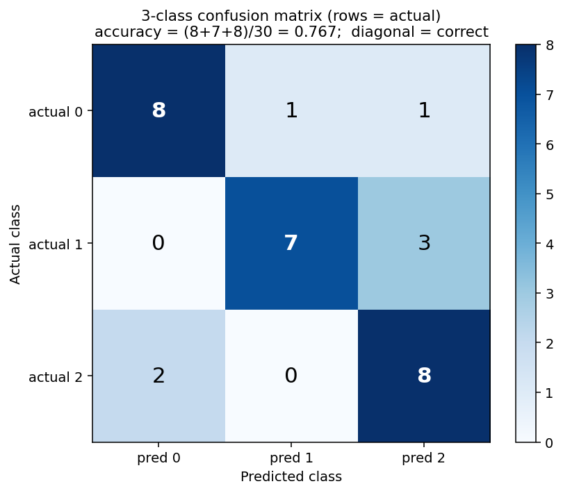
2.14 Confusion matrix and the fallacy of accurate tests¶
For a classifier, the confusion matrix tabulates actual class (rows) vs predicted class (columns); the diagonal holds the correct predictions. From it: accuracy, sensitivity, specificity, prevalence (§4.13). The lecture's warning — the fallacy of accurate tests: a COVID test with 99 % accuracy in a population with 1 % prevalence gives 99 true positives but also 99 false positives → if your test is positive, it is wrong half the time. Accuracy alone is meaningless without prevalence.
বাংলা: Confusion matrix-এ সারি = আসল class, কলাম = predicted class; কর্ণ (diagonal) বরাবর সংখ্যাগুলোই সঠিক prediction। এ থেকেই accuracy, sensitivity, specificity, prevalence বের হয়। Lecture-এর বিখ্যাত সতর্কবাণী: ৯৯% accurate COVID test-ও যদি এমন জনগোষ্ঠীতে চালাও যেখানে মাত্র ১% মানুষ আক্রান্ত, তাহলে positive ফলের অর্ধেকই ভুল! কারণ ৯৯ জন সত্যিকারের রোগীর পাশে ৯,৯০০ সুস্থ মানুষের ১% = ৯৯ জনও ভুল করে positive হয়। শিক্ষা: prevalence না জেনে accuracy-র কথা শুনে ভুলো না।
2.15 The ML pipeline (lecture's step-by-step guide)¶
ML is no black box — it needs careful planning. The lecture's six steps, demonstrated on two end-to-end examples (housing-price regression and iris-flower classification):
- Framing — what is observed, what answer do you want to predict? (Housing: inputs ℝᴺ census parameters → output ℝ median price. Flowers: input image → output ℝ³ class probabilities, because "an integer 1–3" is a bad output choice.)
- Data collection — collect, clean, prepare; remove broken entries (
isnan). - Data analysis — visualize, look for biases and correlations; check if a simpler non-ML technique suffices.
- Feature processing — normalize to [0,1]: \((x - x.\min ()) / (x.\max () - x.\min ())\), or standardize: \((x - x.mean()) / x.\operatorname{std}()\); log-transform high-dynamic-range data; networks cannot handle strong variance in the data.
- Model building — choose architecture and loss; start simple (e.g. two dense hidden layers of 32 ReLU units).
- Training, then prediction — fit on training data, monitor train/validation curves, finally run inference on new data.
Also remember the terminology synonyms (communities differ): features = attributes = x; output = labels = ground truth = reference = y; network = model; loss = metric = cost = error; training = fitting = optimization; evaluation = performance; prediction = inference.
বাংলা: ML কোনো black box নয় — ছয়টা ধাপে পরিকল্পনা করতে হয়: (১) framing — কী দেখে কী অনুমান করবে; (২) data সংগ্রহ ও পরিষ্কার; (৩) data বিশ্লেষণ — bias আছে কি না দেখো; (৪) feature processing — [0,1]-এ normalize বা mean-0/std-1 standardize; (৫) model building — সরল architecture দিয়ে শুরু; (৬) training ও prediction। আর synonym-গুলো চিনে রাখো: feature = attribute = x; label = ground truth = y; loss = cost = error; training = fitting; prediction = inference — বিভিন্ন community ভিন্ন শব্দ ব্যবহার করে, জিনিস একই।
§3 Vocabulary Table¶
| Term | Simple English | বাংলা ব্যাখ্যা | Example |
|---|---|---|---|
| Feature | One input variable | একটি input বৈশিষ্ট্য — model যা দেখে | petal length of a flower |
| Label / ground truth | The desired correct output | কাঙ্ক্ষিত সঠিক উত্তর, যা দিয়ে শেখানো হয় | "iris-setosa", digit "7" |
| Dataset | Collection of (input, label) pairs | (input, label) জোড়ার সংগ্রহ | MNIST: 70,000 digit images |
| Hypothesis / model | The parametrised function we fit | যে function-এর parameter আমরা শেখাই | \(f(x) = Wx + b\) |
Weights W |
Numbers the network learns | Network যে সংখ্যাগুলো শেখে | every \(w_{ij}\) entry |
Bias b |
Constant added inside a neuron | Neuron-এর ভেতরে যোগ হওয়া ধ্রুবক, রেখাকে সরায় | the +b term |
| Parameters | All learnable numbers (weights + biases) | শেখার যোগ্য সব সংখ্যা একসাথে | 9,098 in our tiny CNN |
| Hyperparameter | Setting chosen by you, not learned | তুমি নিজে ঠিক করো, network শেখে না | η, batch size, #layers |
| Activation function | Non-linear function applied per neuron | প্রতিটি neuron-এ বসানো non-linear function | ReLU, sigmoid, softmax |
| Logits | Raw scores before softmax | Softmax-এর আগের কাঁচা score (যেকোনো বাস্তব সংখ্যা) | \(z = (2.0, 1.0, 0.1)\) |
| Loss function | Measures how wrong predictions are | Prediction কতটা ভুল তা মাপে — ছোট মানেই ভালো | MSE, cross-entropy |
| Gradient | Vector of steepest increase of loss | Loss সবচেয়ে দ্রুত যেদিকে বাড়ে সেই দিক | \(\partial L/\partial w\) |
| Gradient descent | Step against the gradient to lower loss | Gradient-এর উল্টো দিকে হেঁটে loss কমানো | \(w \leftarrow w - \eta \cdot \partial L/\partial w\) |
| Learning rate η | Step size of each update | প্রতি update-এ পদক্ষেপের আকার | 0.001 |
| Backpropagation | Chain-rule recipe for all gradients | Chain rule দিয়ে সব gradient একসাথে বের করার কৌশল | PyTorch loss.backward() |
| Epoch | One full pass over the training data | পুরো training data-র একটি সম্পূর্ণ চক্র | "train for 100 epochs" |
| Batch / mini-batch | Samples processed per weight update | এক update-এ কতগুলো sample দেখা হয় | batch_size = 32 |
| Iteration | One weight update (one batch) | একটি batch = একটি update | 1 epoch = ⌈N/B⌉ iterations |
| One-hot encoding | Class as a 0/1 indicator vector | Class-কে 0/1 vector-এ লেখা — সঠিক জায়গায় 1 | class 1 of 3 → (0, 1, 0) |
| Overfitting | Memorising training data, failing on new data | Training data মুখস্থ, নতুন data-তে ব্যর্থ | val loss rises, train falls |
| Underfitting | Model too simple even for training data | Model এত সরল যে train data-ও শিখতে পারে না | line fit on a sine curve |
| Regularization | Any trick that fights overfitting | Overfitting ঠেকানোর যে কোনো কৌশল | L2, dropout, early stop |
| Weight decay (L2) | Penalty on large weights | বড় weight-এর জন্য জরিমানা — weight ছোট রাখে | \(+ (\lambda /2)\|w\|^{2}\) in loss |
| Dropout | Randomly disable neurons while training | Training-এ এলোমেলোভাবে কিছু neuron বন্ধ রাখা | p = 0.5 |
| Early stopping | Stop when validation loss starts rising | Validation loss বাড়তে শুরু করলেই থামা | Figure 4 green line |
| Data augmentation | Artificially enlarge training data | ঘুরিয়ে/উল্টে/কেটে কৃত্রিমভাবে data বাড়ানো | random flips, crops |
| Train/val/test split | Three separate roles for data | Data-র তিনটি আলাদা ভূমিকা: শেখা/বাছাই/চূড়ান্ত যাচাই | 80 / 10 / 10 |
| K-fold cross-validation | Rotate K groups as test set | K ভাগের প্রতিটা একবার test হয়, ফলের গড় নেওয়া হয় | K = 5 |
| k-NN | Vote among k closest training points | সবচেয়ে কাছের k-টা প্রতিবেশীর সংখ্যাগরিষ্ঠ ভোট | k = 3, Euclidean |
| Convolution layer | Learned filter slid over the image | শেখা filter যা পুরো ছবির ওপর একইভাবে চলে | 3×3 kernel, 8 filters |
| Kernel / filter | The small weight window of a conv layer | Conv layer-এর ছোট weight জানালা | 3×3, 5×5 |
| Feature map | Output image of one conv filter | একটি filter-এর output ছবি | 28×28×8 after conv1 |
| Stride S | Step of the sliding window | জানালা প্রতিবার কত ঘর সরে | S = 1 or 2 |
| Padding P | Zeros added around the border | কিনারায় শূন্য বসানো যাতে আকার ঠিক থাকে | P = 1 keeps 3×3 size |
| (Max-)Pooling | Downsample by keeping the max | 2×2 ব্লকের সর্বোচ্চ মান রেখে ছবি অর্ধেক করা | 2×2 max-pool |
| Fully-connected (dense) layer | Every input connects to every output | প্রতিটি input প্রতিটি output-এর সাথে যুক্ত | 784 → 10 |
| Latent space | Compressed internal representation | Autoencoder-এর মাঝের সংকুচিত উপস্থাপনা | bottleneck vector |
| Confusion matrix | Table of actual vs predicted classes | আসল বনাম predicted class-এর টেবিল | 3×3 matrix in Q3a |
| Accuracy | Fraction of all predictions correct | মোট prediction-এর কত ভাগ সঠিক | diagonal / total |
| Sensitivity (recall) | Fraction of real positives found | আসল positive-দের কত ভাগ ধরা পড়লো | TP / (TP + FN) |
| Specificity | Fraction of real negatives found | আসল negative-দের কত ভাগ ঠিক চেনা গেলো | TN / (TN + FP) |
| Prevalence | Fraction of positives in the data | Data-তে positive class-এর অনুপাত | (TP + FN) / total |
| Inference / prediction | Using the trained model on new data | শেখা শেষে নতুন data-তে model চালানো | model.predict(x) |
| Transfer learning | Reuse a model trained on another task | অন্য কাজে শেখা model নতুন কাজে লাগানো | pretrained Faster R-CNN |
| Vanishing gradient | Gradient shrinks towards early layers | পেছনের layer-এ যেতে যেতে gradient ক্ষুদ্র হয়ে যাওয়া | sigmoid chains, σ′ ≤ 0.25 |
| Batch normalization | Normalize activations per mini-batch | প্রতি mini-batch-এ activation-কে normalize করা | mean 0, var 1, then γ, β |
§4 Mathematical Foundations¶
Every formula in this section uses plain unicode math (no LaTeX). Each subsection follows the same drill: formula → symbols → derivation → worked numbers → বাংলা intuition. Work through these with pen and paper — the Tier-C exam questions in §8 are exactly these computations with different numbers.
4.1 The supervised-learning setup¶
Dataset:     D = { (x⁽¹⁾, y⁽¹⁾), (x⁽²⁾, y⁽²⁾), …, (x⁽ᴺ⁾, y⁽ᴺ⁾) }
Hypothesis:  f_θ : ℝⁿ → ℝᵐ          (a parametrised function, θ = all weights)
Loss:        L(θ) = (1/N) Σᵢ ℓ( f_θ(x⁽ⁱ⁾), y⁽ⁱ⁾ )
Goal:        θ* = argmin_θ L(θ)
| Symbol | Meaning |
|---|---|
| \(x^{(i)} \in \mathbb{R}^{n}\) | i-th input (feature vector, n features) |
| \(y^{(i)} \in \mathbb{R}^{m}\) | i-th label / ground truth (m outputs) |
N |
number of training samples |
| \(f_\theta\) | the model (hypothesis); θ collects every weight and bias |
ℓ(ŷ, y) |
per-sample loss comparing prediction ŷ with truth y |
| \(L(\theta )\) | total (average) loss over the dataset |
| \(\operatorname{argmin}_\theta\) | "the θ that makes L smallest" |
Interpretation. Learning = an optimization problem. We choose a family of functions (the architecture fixes the form of \(f_\theta\)), and training searches inside that family for the member \(\theta *\) whose predictions disagree least with the labels. Regression: \(m = 1\), y is a real number, ℓ is usually squared error. Classification with K classes: \(m = K\), y is one-hot, ℓ is cross-entropy.
Worked micro-example. Predict exam points y from study hours x. Dataset \(D = {(1, 2), (2, 3)}\) (N = 2, n = m = 1). Hypothesis family: all lines \(f_\theta (x) = w\cdot x + b\), so \(\theta = (w, b)\). The loss landscape L(w, b) is a 2-D surface; training = finding its lowest point. This exact tiny dataset is reused for the gradient-descent computation in §4.7.
বাংলা: Supervised learning মানে আসলে একটা optimization সমস্যা। আমাদের কাছে আছে N-টা (input, সঠিক উত্তর) জোড়া। আমরা একটা function-পরিবার বেছে নিই (যেমন: সব সরলরেখা wx + b), যার নিয়ন্ত্রণযোগ্য সংখ্যাগুলো হলো parameter θ। Loss function \(L(\theta )\) মাপে এই function-টা সব উদাহরণ মিলিয়ে গড়ে কতটা ভুল করছে। Training মানে θ-এর সেই মানটা খোঁজা যেখানে L সবচেয়ে ছোট — অর্থাৎ argmin। পুরো deep learning এই এক লাইনের গল্প: ভুল মাপো, ভুল কমাও।
4.2 Linear classifier / regressor: y = Wx + b (with shapes!)¶
Single output (line):        ŷ = w·x + b                    w, x ∈ ℝⁿ,  b, ŷ ∈ ℝ
Multiple outputs (layer):    ŷ = W·x + b                    W ∈ ℝ^(m×n), x ∈ ℝⁿ, b, ŷ ∈ ℝᵐ
Element form:                ŷᵢ = Σⱼ Wᵢⱼ·xⱼ + bᵢ            i = 1…m,  j = 1…n
| Symbol | Meaning | Shape |
|---|---|---|
x |
input feature vector | n × 1 |
W |
weight matrix (row i = weights of output neuron i) | m × n |
b |
bias vector | m × 1 |
ŷ |
prediction | m × 1 |
Shape rule to memorize: \((m \times n) \cdot (n \times 1) + (m \times 1) = (m \times 1)\). The inner dimension n must match; the parameter count of this layer is \(m\cdot n + m = m(n + 1)\).
Lecture connection. The lecture shows that the school line \(y = ax + b\) is a perceptron: take inputs \(x_{1} = x\) and a constant \(x_{2} = 1\) with weights \(w_{11} = a\), \(w_{12} = b\); then \(l = w_{11}\cdot x_{1} + w_{12}\cdot x_{2} = ax + b\), writable as the matrix product \((w_{11} w_{12})\cdot (x_{1}, x_{2})^{T}\). The bias is just a weight attached to a constant-1 input.
Worked example. n = 3 features, m = 2 outputs:
W = ⎛ 1   0  −1 ⎞      x = (2, 1, 1)ᵀ       b = (0.5, −1)ᵀ
    ⎝ 2   1   0 ⎠

ŷ₁ = 1·2 + 0·1 + (−1)·1 + 0.5 = 2 − 1 + 0.5 = 1.5
ŷ₂ = 2·2 + 1·1 +   0·1  + (−1) = 4 + 1 − 1   = 4.0
ŷ = (1.5, 4.0)ᵀ          parameters: 2·3 + 2 = 8
For a classifier, the entries of ŷ are the logits (class scores); the predicted class is the argmax (or we convert to probabilities via softmax, §4.5). A single linear layer can only carve the input space with straight hyperplanes — Figure 1 shows where that works and where (XOR) it provably fails.
বাংলা: \(\hat{y} = Wx + b\) হলো deep learning-এর মৌলিক ইট। Shape মুখস্থ রাখো: W হলো (m×n) — m-টা output neuron-এর প্রতিটার জন্য এক সারি weight; x হলো (n×1) input; b হলো (m×1) bias। ভেতরের মাত্রা n দুই পাশে মিলতেই হবে। এই layer-এর parameter সংখ্যা = m·(n+1) — exam-এ parameter গোনার প্রশ্নে এই সূত্রই বারবার লাগবে। আর মনে রাখো: bias আসলে বিশেষ কিছু না — ধ্রুবক-1 input-এর সাথে লাগানো একটা weight মাত্র। একটা linear layer একা শুধু সোজা hyperplane দিয়ে জগৎ ভাগ করতে পারে — XOR-এর মতো আড়াআড়ি pattern পারে না, তাই non-linearity লাগে।
4.3 MSE loss and its gradient — full derivation¶
| Symbol | Meaning |
|---|---|
| \(\hat{y}^{(i)}\) | model prediction for sample i |
| \(y^{(i)}\) | true value for sample i |
| \(\hat{y}^{(i)} - y^{(i)}\) | the residual (signed error) of sample i |
E |
mean of squared residuals — always ≥ 0, equals 0 only for a perfect fit |
Why squared? (i) sign disappears — overshoot and undershoot both count; (ii) large errors are punished quadratically; (iii) E is smooth and differentiable, perfect for gradient descent. (The lecture notes that for the purely linear case a closed-form least-squares solution exists — gradient descent here is to convey the general idea.)
Derivation of the gradient. Apply the chain rule to each summand. Let \(r_{i} = \hat{y}^{(i)} - y^{(i)} = w\cdot x^{(i)} + b - y^{(i)}\):
∂E/∂w = (1/N) Σᵢ ∂(rᵢ²)/∂w
      = (1/N) Σᵢ 2·rᵢ · ∂rᵢ/∂w          (chain rule, outer: square)
      = (1/N) Σᵢ 2·rᵢ · x⁽ⁱ⁾             (inner: ∂(w·x⁽ⁱ⁾ + b − y⁽ⁱ⁾)/∂w = x⁽ⁱ⁾)
      = (2/N) Σᵢ ( ŷ⁽ⁱ⁾ − y⁽ⁱ⁾ ) · x⁽ⁱ⁾

∂E/∂b = (1/N) Σᵢ 2·rᵢ · ∂rᵢ/∂b = (2/N) Σᵢ ( ŷ⁽ⁱ⁾ − y⁽ⁱ⁾ )        (since ∂rᵢ/∂b = 1)
Reading the result: the gradient w.r.t. w is the residual-weighted average of the inputs; the gradient w.r.t. b is just the average residual (×2). If predictions are too small (residuals negative), the gradients are negative → gradient descent will push w and b up. The mechanism is self-correcting.
Worked example. Data \(D = {(1, 2), (2, 3)}\), current parameters \(w = 0.5\), \(b = 0\):
Both gradients are negative → both parameters must increase to reduce the loss. Exactly what intuition says: the line 0.5x lies far below the points (1,2) and (2,3).
বাংলা: MSE মানে ভুলের বর্গের গড়। বর্গ করার তিনটা কারণ: চিহ্ন মুছে যায় (উপরে-নিচে দুই ভুলই সমান দোষ), বড় ভুল বেশি শাস্তি পায়, আর function-টা মসৃণ থাকে বলে derivative নেওয়া যায়। Gradient-এর সূত্র দুটো মুখস্থ নয়, বুঝে রাখো: ∂E/∂w = (2/N)·Σ(residual × input) আর \(\partial E/\partial b = (2/N)\cdot \Sigma (residual)\)। Residual ঋণাত্মক মানে prediction ছোট হচ্ছে — তখন gradient ঋণাত্মক, আর gradient descent ঋণাত্মক gradient-এর উল্টো দিকে হাঁটে বলে w আর b বেড়ে যায় — অর্থাৎ system নিজে নিজেই ভুল শুধরে নেয়। এটাই পুরো training-এর হৃদয়।
4.4 Sigmoid and its derivative — full derivation¶
Sigmoid:      σ(x) = 1 / (1 + e⁻ˣ)
Derivative:   σ′(x) = σ(x) · (1 − σ(x))
Properties:   σ: ℝ → (0, 1),  σ(0) = 0.5,  σ(−x) = 1 − σ(x),  max σ′ = σ′(0) = 0.25
| Symbol | Meaning |
|---|---|
| \(e^{-x}\) | exponential decay; huge for x ≪ 0, tiny for x ≫ 0 |
| \(\sigma (x)\) | squashes any real number into (0, 1) → usable as a probability |
| \(\sigma '(x)\) | slope; bell-shaped, peaks at 0.25, ≈ 0 in the saturated tails |
Derivation of σ′ = σ(1 − σ). Write \(\sigma (x) = (1 + e^{-x})^{-1}\) and use the chain rule:
σ′(x) = −(1 + e⁻ˣ)⁻² · d(1 + e⁻ˣ)/dx
      = −(1 + e⁻ˣ)⁻² · (−e⁻ˣ)
      = e⁻ˣ / (1 + e⁻ˣ)²

Now split the fraction:
      = [ 1 / (1 + e⁻ˣ) ] · [ e⁻ˣ / (1 + e⁻ˣ) ]
      = σ(x) · [ (1 + e⁻ˣ − 1) / (1 + e⁻ˣ) ]
      = σ(x) · [ 1 − 1/(1 + e⁻ˣ) ]
      = σ(x) · ( 1 − σ(x) )                                            ∎
This identity is gold for backpropagation: once the forward pass computed \(h = \sigma (z)\), the local gradient is simply \(h\cdot (1 - h)\) — no extra exponentials needed.
Worked numbers.
σ(0)   = 1/(1+1)        = 0.5          σ′(0)   = 0.5·0.5     = 0.25  (the maximum!)
σ(0.5) = 1/(1+0.6065)   = 0.6225       σ′(0.5) = 0.6225·0.3775 = 0.2350
σ(2)   = 1/(1+0.1353)   = 0.8808       σ′(2)   = 0.8808·0.1192 = 0.1050
σ(5)   ≈ 0.9933                        σ′(5)   ≈ 0.0066   ← saturation: gradient nearly dead
Vanishing-gradient preview (Tier D!). Since \(\sigma ' \le 0.25\) everywhere, a chain of 10 sigmoid layers multiplies gradients by at most \(0.25^{10} \approx 9.5\cdot 10^{-7}\) — early layers receive essentially no learning signal. ReLU (\(derivative = 1\) for positive inputs) fixes this; see Figure 3 and mock question D1.
বাংলা: Sigmoid যে কোনো বাস্তব সংখ্যাকে চেপে (0,1)-এর ভেতরে আনে — তাই output-কে probability হিসেবে পড়া যায়। সবচেয়ে দরকারি ফল: \(\sigma ' = \sigma (1-\sigma )\) — অর্থাৎ forward pass-এ σ-এর মান একবার বের করলেই derivative প্রায় বিনা খরচে পাওয়া যায়, backpropagation-এ এটাই ব্যবহার হয়। কিন্তু লক্ষ করো: σ′-এর সর্বোচ্চ মান মাত্র 0.25, আর |x| বড় হলে σ′ প্রায় শূন্য (saturation)। ফলে অনেকগুলো sigmoid layer-এর ভেতর দিয়ে gradient পেছনে যেতে যেতে 0.25-এর ঘাতে গুণ হয়ে কার্যত মরে যায় — এটাই vanishing gradient। ReLU-র derivative ধনাত্মক দিকে পুরো 1, তাই সে এই সমস্যা থেকে বাঁচায়।
4.5 Softmax — formula, properties, worked 3-class example¶
| Symbol | Meaning |
|---|---|
| \(z_{i}\) | raw score (logit) of class i — any real number |
| \(e^(z_{i})\) | makes every score positive and exaggerates differences |
| \(\Sigma _{j} e^(z_{j})\) | normalizer: forces the outputs to sum to 1 |
| \(\operatorname{softmax}(z)_{i}\) | probability assigned to class i |
Properties (provable, exam-ready):
- Range: every output ∈ (0, 1) — numerator and denominator are positive, numerator < denominator.
- Sums to one: \(\Sigma _{i} \operatorname{softmax}(z)_{i} = \Sigma _{i} e^(z_{i}) / \Sigma _{j} e^(z_{j}) = 1\) → a valid probability distribution.
- Order-preserving: bigger logit → bigger probability (e^x is monotone); argmax is unchanged.
- Invariance to constant shift: for any constant c,
Practical use: implementations always compute \(\operatorname{softmax}(z - \max (z))\) — same result, but no overflow from huge exponentials (numerical stability).
- Not scale-invariant: multiplying z by a constant does change the output — that is the temperature idea (mock question D3): \(\operatorname{softmax}(z/T)\) is sharper for T < 1, flatter for T > 1.
Worked 3-class example. Logits \(z = (2.0, 1.0, 0.1)\):
e^2.0 = 7.389      e^1.0 = 2.718      e^0.1 = 1.105
Σ = 7.389 + 2.718 + 1.105 = 11.212

p₁ = 7.389/11.212 = 0.659
p₂ = 2.718/11.212 = 0.242
p₃ = 1.105/11.212 = 0.099            check: 0.659 + 0.242 + 0.099 = 1.000 ✓
Shift-invariance check — subtract c = 2 from every logit: \(z' = (0, -1, -1.9)\):
e^0 = 1.000      e^−1 = 0.368      e^−1.9 = 0.150      Σ = 1.518
p′ = (1.000/1.518, 0.368/1.518, 0.150/1.518) = (0.659, 0.242, 0.099)   — identical ✓
See Figure 6 for the bar-chart view including temperature.
বাংলা: Softmax কাঁচা score (logit)-গুলোকে একটা বৈধ probability distribution-এ রূপান্তর করে: প্রতিটা মান (0,1)-এ থাকে আর সব মিলে ঠিক 1 হয়। \(e^x\) ব্যবহারের কারণ — সব মান ধনাত্মক হয়ে যায় আর বড় score-এর প্রাধান্য বাড়ে, কিন্তু ক্রম (কোনটা বড়) বদলায় না। সবচেয়ে গুরুত্বপূর্ণ ধর্ম: সব logit থেকে একই ধ্রুবক c বিয়োগ করলে softmax-এর ফল এতটুকুও বদলায় না — প্রমাণটা এক লাইনের: উপরে-নিচে \(e^c\) কেটে যায়। এই ধর্মেরই বাস্তব প্রয়োগ: overflow এড়াতে সবাই \(z - \max (z)\) দিয়ে হিসাব করে। হাতের উদাহরণটা ((2.0, 1.0, 0.1) → (0.659, 0.242, 0.099)) নিজে একবার calculator-এ মিলিয়ে নাও — exam-এ ঠিক এই ধরনের সংখ্যা আসবে।
4.6 Cross-entropy loss — and why it pairs with softmax¶
One-hot label:    y = (y₁, …, y_K),   y_c = 1 for the true class c, all others 0
Cross-entropy:    L_CE(p, y) = − Σₖ yₖ · ln(pₖ)  =  − ln(p_c)
| Symbol | Meaning |
|---|---|
| \(p = \operatorname{softmax}(z)\) | predicted class probabilities |
y |
one-hot ground truth |
| \(p_{c}\) | probability the model gave to the correct class |
ln |
natural logarithm |
Behaviour: the loss only looks at the probability of the correct class. \(p_{c} = 1 \to L = 0\) (perfect); \(p_{c} = 0.5 \to L = 0.69\); \(p_{c} = 0.01 \to L = 4.61\) (confidently wrong → huge punishment). This is the negative log-likelihood of the data under the model — minimizing cross-entropy = maximum-likelihood estimation for a categorical distribution.
The famous gradient: p − y (derivation sketch). Feed logits z through softmax into cross-entropy. Write the loss directly in terms of z:
L = − ln( softmax(z)_c )
  = − ln( e^(z_c) / Σⱼ e^(zⱼ) )
  = − z_c + ln( Σⱼ e^(zⱼ) )                       (log of quotient)

∂L/∂zᵢ = − ∂z_c/∂zᵢ + ∂/∂zᵢ [ ln Σⱼ e^(zⱼ) ]
       = − δᵢ_c + e^(zᵢ) / Σⱼ e^(zⱼ)              (chain rule on the log-sum)
       = pᵢ − yᵢ                                   ∎

(δᵢ_c = 1 if i = c, else 0 — exactly the one-hot entry yᵢ)
Why this matters (Tier D!): the messy pieces — softmax's Jacobian \(\partial p_{i}/\partial z_{j} = p_{i}(\delta _{ij} - p_{j})\) and the log's \(1/p_{c}\) — cancel perfectly, leaving the cleanest possible error signal: predicted probability minus truth. The gradient is large exactly when the model is badly wrong and never saturates the way MSE + sigmoid does (where an extra σ′ factor kills the gradient for confident-but-wrong outputs). That is why classification uses softmax + cross-entropy, not MSE — see mock question D2.
Worked example. Continue §4.5: \(p = (0.659, 0.242, 0.099)\), true class = class 1 → \(y = (1, 0, 0)\):
Reading: push z₁ up (negative gradient component), push z₂ and z₃ down — in proportion to how much probability they wrongly received. If instead the true class were class 2: \(L = -\ln (0.242) = 1.417\) (worse, as expected).
Implementation warning (classic silent bug): nn.CrossEntropyLoss in PyTorch and SparseCategoricalCrossentropy(from_logits=True) in Keras already include the softmax — feed them raw logits. Applying softmax twice trains, but badly.
বাংলা: Cross-entropy শুধু একটা সংখ্যার দিকে তাকায় — সঠিক class-কে model কত probability দিয়েছে (p_c), আর loss হলো \(-\ln (p_{c})\)। সঠিক class-এ পুরো আস্থা (p_c = 1) হলে loss শূন্য; আত্মবিশ্বাসের সাথে ভুল (p_c ≈ 0) হলে loss আকাশছোঁয়া। আসল জাদুটা gradient-এ: softmax আর cross-entropy একসাথে চালালে জটিল সব derivative কেটেকুটে গিয়ে পড়ে থাকে শুধু \(p - y\) — অর্থাৎ "অনুমান বিয়োগ সত্য"। ভুল যত বড়, সংশোধনের ধাক্কা তত জোরালো, আর কখনো saturate করে না — এই কারণেই classification-এ MSE নয়, softmax + cross-entropy-ই মানক জুটি। আর practical সতর্কতা: PyTorch-এর CrossEntropyLoss-এর ভেতরে softmax আগে থেকেই আছে — নিজে আরেকবার softmax লাগালে নিঃশব্দ bug হবে।
4.7 Gradient descent — update rule, learning rate, one full hand-computed step¶
| Symbol | Meaning |
|---|---|
| \(\theta _{t}\) | parameter value at step t |
| \(\eta\) | learning rate (step size), e.g. 0.001 … 0.1 |
| \(\partial L/\partial \theta\) | gradient of the loss, evaluated at the current parameters |
| minus sign | gradient points uphill; we walk downhill |
Learning-rate effects (Figure 2). For the quadratic toy loss \(L(w) = \tfrac{1}{2}\cdot a\cdot w^{2}\) the gradient is \(a\cdot w\), so one update gives \(w \leftarrow (1 - \eta \cdot a)\cdot w\):
|1 − η·a| < 1   → converges          (smooth if 0 < η·a < 1, oscillating if 1 < η·a < 2)
|1 − η·a| > 1   → DIVERGES           (η too large: each step overshoots farther)
η tiny          → converges but painfully slowly
This is why the lecture says: "if too strong, the net will not converge; if too weak, learning will be slow." Variants used in practice: SGD with mini-batches (gradient from a random batch — noisy but cheap), Momentum, RMSProp (the lecture's housing example uses RMSProp), Adam (momentum + adaptive step sizes).
One full hand-computed step. Model \(\hat{y} = w\cdot x + b\), data \(D = {(1, 2), (2, 3)}\), start \(w_{0} = 0, b_{0} = 0\), learning rate \(\eta = 0.1\), loss = MSE (gradients from §4.3).
Step 0 — forward:
  ŷ⁽¹⁾ = 0·1 + 0 = 0       r₁ = 0 − 2 = −2
  ŷ⁽²⁾ = 0·2 + 0 = 0       r₂ = 0 − 3 = −3
  E₀ = (1/2)( (−2)² + (−3)² ) = (4 + 9)/2 = 6.5

Step 0 — gradients:
  ∂E/∂w = (2/2)·( (−2)·1 + (−3)·2 ) = −2 − 6 = −8
  ∂E/∂b = (2/2)·( −2 + (−3) )       = −5

Step 0 — update:
  w₁ = 0 − 0.1·(−8) = 0.8
  b₁ = 0 − 0.1·(−5) = 0.5

Verify the loss dropped:
  ŷ⁽¹⁾ = 0.8·1 + 0.5 = 1.3     r₁ = −0.7
  ŷ⁽²⁾ = 0.8·2 + 0.5 = 2.1     r₂ = −0.9
  E₁ = ( 0.49 + 0.81 )/2 = 0.65          ← loss fell 6.5 → 0.65 (10× better!)
Second step (to see the process settle):
  ∂E/∂w = (2/2)( (−0.7)·1 + (−0.9)·2 ) = −0.7 − 1.8 = −2.5
  ∂E/∂b = (2/2)( −0.7 − 0.9 )          = −1.6
  w₂ = 0.8 + 0.1·2.5  = 1.05
  b₂ = 0.5 + 0.1·1.6  = 0.66
  New predictions: 1.71 and 2.76  →  E₂ = ( (−0.29)² + (−0.24)² )/2 = 0.0709
The parameters head toward the perfect line \(y = x + 1\) (which fits both points exactly, E = 0). Notice the gradients shrink as we approach the minimum — steps become automatically smaller even with fixed η.
বাংলা: Update-এর সূত্র একটাই: নতুন weight = পুরনো weight − η × gradient। Minus চিহ্নটা প্রাণ — gradient দেখায় কোন দিকে loss বাড়ে, আমরা হাঁটি তার উল্টো দিকে। Learning rate η-এর তিন অবস্থা মুখস্থ রাখো: ঠিকঠাক হলে মসৃণ convergence, খুব বড় হলে প্রতি লাফে উপত্যকা পেরিয়ে আরো দূরে গিয়ে পড়ে (diverge), খুব ছোট হলে পৌঁছাবে কিন্তু হাজার বছর লাগবে। উপরের হাতে-করা হিসাবটা খাতায় নিজে একবার তোলো: শূন্য থেকে শুরু করে এক step-এই loss 6.5 থেকে 0.65-এ নেমে গেছে, আর w, b এগোচ্ছে নিখুঁত রেখা y = x + 1-এর দিকে। আরেকটা সূক্ষ্ম পর্যবেক্ষণ: minimum-এর কাছে যেতে যেতে gradient নিজেই ছোট হয়ে আসে, তাই η একই থাকলেও পদক্ষেপ ছোট হতে থাকে।
4.8 Backpropagation — a 2-layer network worked end-to-end with real numbers¶
The network (scalar everywhere, so every step is checkable by hand):
x ──→ [ z₁ = w₁·x + b₁ ] ──→ [ h = σ(z₁) ] ──→ [ ŷ = w₂·h + b₂ ] ──→ L = ½·(ŷ − y)²
        layer 1 (linear)       activation        layer 2 (linear)        loss
Chain rule along the graph (memorize the pattern, not the numbers):
∂L/∂ŷ  = ŷ − y                                  (derivative of ½(ŷ−y)²)
∂L/∂w₂ = ∂L/∂ŷ · h                              (ŷ = w₂h + b₂ ⇒ ∂ŷ/∂w₂ = h)
∂L/∂b₂ = ∂L/∂ŷ · 1
∂L/∂h  = ∂L/∂ŷ · w₂                             (the error flows back through w₂)
∂L/∂z₁ = ∂L/∂h · σ′(z₁) = ∂L/∂h · h(1−h)        (sigmoid local gradient, §4.4)
∂L/∂w₁ = ∂L/∂z₁ · x
∂L/∂b₁ = ∂L/∂z₁ · 1
Numbers. Take \(x = 1, y = 1\), initial \(w_{1} = 0.5, b_{1} = 0, w_{2} = 1, b_{2} = 0\), learning rate \(\eta = 0.5\).
FORWARD PASS (store everything!):
  z₁ = 0.5·1 + 0          = 0.5
  h  = σ(0.5)             = 0.6225
  ŷ  = 1·0.6225 + 0       = 0.6225
  L  = ½·(0.6225 − 1)²    = ½·(−0.3775)² = 0.0713

BACKWARD PASS (output → input):
  ∂L/∂ŷ  = ŷ − y = −0.3775
  ∂L/∂w₂ = −0.3775 · 0.6225          = −0.2350
  ∂L/∂b₂ = −0.3775
  ∂L/∂h  = −0.3775 · 1               = −0.3775
  σ′(z₁) = h(1−h) = 0.6225·0.3775    =  0.2350
  ∂L/∂z₁ = −0.3775 · 0.2350          = −0.0887
  ∂L/∂w₁ = −0.0887 · 1               = −0.0887
  ∂L/∂b₁ = −0.0887

UPDATE (θ ← θ − η·grad, η = 0.5):
  w₂ ← 1   − 0.5·(−0.2350) = 1.1175
  b₂ ← 0   − 0.5·(−0.3775) = 0.1888
  w₁ ← 0.5 − 0.5·(−0.0887) = 0.5444
  b₁ ← 0   − 0.5·(−0.0887) = 0.0444

VERIFY — second forward pass:
  z₁ = 0.5444 + 0.0444 = 0.5887
  h  = σ(0.5887)       = 0.6431
  ŷ  = 1.1175·0.6431 + 0.1888 = 0.9074
  L  = ½·(0.9074 − 1)² = 0.0043          ← loss fell 0.0713 → 0.0043 ✓
Three observations worth exam points. 1. All gradients reuse \(\partial L/\partial \hat{y}\) — computed once, propagated backwards. That sharing is the whole point of backprop (cost ≈ 2 forward passes, not one pass per weight). 2. The gradient reaching layer 1 has been multiplied by \(\sigma '(z_{1}) = 0.235 < 0.25\). Stack ten such layers and the front of the network learns ~\(0.25^{10} \approx 10^{-6}\) times slower — the vanishing gradient problem, the lecture's "the deeper the net, the more problematic this becomes (diminishing gradient)". 3. Layer-2 parameters got bigger updates than layer-1 parameters — typical: late layers learn fastest.
বাংলা: Backpropagation-এর পুরো রহস্য এই worked example-এ। নিয়মটা ছন্দের মতো: forward pass-এ সব মাঝের মান জমাও, backward pass-এ output থেকে পেছনে এসে প্রতি ধাপে local derivative গুণ করো। খেয়াল করো \(\partial L/\partial \hat{y} = -0.3775\) একবারই হিসাব হয়েছে, তারপর সেটাই সব weight-এর gradient-এ ভাগ বসিয়েছে — এই পুনঃব্যবহারই backprop-কে দ্রুত করে। আরো দেখো: layer 1-এ পৌঁছানো gradient-কে σ′ = 0.235 দিয়ে গুণ খেতে হয়েছে, মানে সামনের layer-এর শেখার সংকেত এক ধাপেই চার ভাগের এক ভাগ হয়ে গেছে — দশ layer হলে কার্যত শূন্য। Update-এর পর আবার forward pass চালিয়ে দেখো loss 0.0713 → 0.0043 — পদ্ধতিটা কাজ করছে, এই যাচাইটাই exam-এ পুরো নম্বর আনে।
4.9 Train / validation / test — the mathematics of honest evaluation¶
D = D_train ∪ D_val ∪ D_test          (disjoint!)
typical sizes:  80% / 10% / 10%   or  60% / 20% / 20%

Normalization (computed on D_train ONLY, then applied everywhere):
  min-max:      x′ = (x − min_train) / (max_train − min_train)        → range [0, 1]
  standardize:  x′ = (x − μ_train) / σ_train                          → mean 0, std 1
Roles: \(D_{train}\) fits the weights; \(D_{val}\) selects hyperparameters and triggers early stopping; \(D_{test}\) is used exactly once for the final report. Using test data for any decision = information leak = your reported number is a lie.
K-fold cross-validation (small datasets): partition D into K equal folds; for k = 1…K train on the other K−1 folds and evaluate on fold k; report mean ± std of the K scores. Cost: K trainings; benefit: every sample is tested once, the estimate is far less split-dependent.
Overfitting in curves (Figures 4 and 5): training loss decreases monotonically; validation loss decreases, bottoms out, then rises — the rise marks memorisation. The lecture's housing example also shows an unstable validation curve as a warning sign (could indicate overfitting, or a bad batch size / epoch count).
বাংলা: তিনটা set-এর ভূমিকা আলাদা: train = weight শেখা, validation = hyperparameter বাছাই + early stopping, test = একবারই, শুধু শেষ নম্বরের জন্য। Normalization-এর সূত্রে লক্ষ করো min, max, μ, σ সব শুধু training set থেকে আসছে — তারপর সেই একই সংখ্যা দিয়ে val/test রূপান্তর করা হয়। Test-এর তথ্য কোনো সিদ্ধান্তে ঢুকলেই সেটা leak, আর তোমার report করা score মিথ্যা। ছোট dataset-এ K-fold: K বার train করে প্রতিটা ভাগকে একবার test বানাও — খরচ K গুণ, কিন্তু estimate অনেক নির্ভরযোগ্য। Curve পড়তে শেখো: train নামছে আর validation নেমে গিয়ে আবার উঠছে — ওই ওঠার মুহূর্তটাই overfitting শুরুর ঘণ্টা।
4.10 Regularization — L2 weight decay inside the update rule¶
Regularized loss:    L_total(w) = L_data(w) + (λ/2)·‖w‖²       ‖w‖² = Σᵢ wᵢ²
Gradient:            ∂L_total/∂w = ∂L_data/∂w + λ·w
GD update:           w ← w − η·( ∂L_data/∂w + λ·w )
                       = (1 − η·λ)·w − η·∂L_data/∂w
| Symbol | Meaning |
|---|---|
| \(\lambda\) | regularization strength (a hyperparameter, e.g. 10⁻⁴) |
| \((\lambda /2)\cdot \|w\|^{2}\) | penalty that grows with the squared size of the weights |
| \((1 - \eta \cdot \lambda )\) | the "decay factor" — every step first shrinks w a little |
Why "weight decay": the rewritten update shows each step multiplies the weights by \((1 - \eta \lambda ) < 1\) before applying the usual data gradient — weights continually decay toward 0 unless the data pushes back. Small weights = smoother functions = less capacity to memorise noise = less overfitting. (The factor λ/2 is cosmetic: it cancels the 2 from differentiating the square.)
Worked numbers. \(w = 2, \eta = 0.1, \lambda = 0.1, \partial L_{data}/\partial w = 0.5\):
w ← (1 − 0.1·0.1)·2 − 0.1·0.5 = 0.99·2 − 0.05 = 1.98 − 0.05 = 1.93
(without regularization: w ← 2 − 0.05 = 1.95 — L2 pulled it 0.02 closer to zero)
L1 alternative (Tier D): penalty \(\lambda \cdot \Sigma |w_{i}|\), gradient \(\lambda \cdot \operatorname{sign}(w)\) — subtracts a constant amount each step regardless of size, so small weights get driven exactly to 0 → sparse solutions. Geometric picture: L2's constraint region is a smooth ball (optimum rarely on an axis), L1's is a diamond whose corners sit on the axes (optimum often has zero coordinates). Other regularizers from the lecture: dropout, early stopping, data augmentation, batch normalization (mild effect).
বাংলা: L2 regularization মানে loss-এর সাথে \((\lambda /2)\cdot \|w\|^{2}\) জরিমানা যোগ করা — weight যত বড়, জরিমানা তত বেশি। Update rule-এ এর চেহারা সবচেয়ে সুন্দর: প্রতি ধাপে আগে weight-কে \((1 - \eta \lambda )\) দিয়ে গুণ করা হয়, মানে weight একটু একটু করে শূন্যের দিকে "ক্ষয়" হয় — এজন্যই নাম weight decay। ছোট weight মানে মসৃণ function, মানে noise মুখস্থ করার ক্ষমতা কম, মানে overfitting কম। L1-এর সাথে পার্থক্যটা geometry-তে: L2-এর সীমানা গোল বল (weight ছোট হয় কিন্তু শূন্য হয় না), L1-এর সীমানা হীরার মতো কোণাওয়ালা — কোণাগুলো অক্ষের ওপর বলে অনেক weight ঠিক শূন্য হয়ে যায় (sparsity)।
4.11 k-Nearest Neighbours — distance, vote, bias–variance¶
Distance:   d(q, x⁽ⁱ⁾) = √( Σ_j ( q_j − x⁽ⁱ⁾_j )² )            (Euclidean)
Rule:       find the k training points with smallest d(q, ·)
            ŷ(q) = majority class among those k neighbours
            (regression variant: average of the k neighbours' values)
| Symbol | Meaning |
|---|---|
q |
query point to classify |
| \(x^{(i)}\) | stored training points (k-NN keeps them ALL — "lazy learning") |
k |
number of neighbours consulted (odd k avoids ties in 2-class problems) |
Worked example. Training set: \(A = (1,1)\) red, \(B = (2,2)\) red, \(C = (5,5)\) blue, \(D = (6,5)\) blue. Query \(q = (3,2)\), k = 3:
d(q,A) = √((3−1)² + (2−1)²) = √5  = 2.236
d(q,B) = √((3−2)² + (2−2)²) = √1  = 1.000
d(q,C) = √((3−5)² + (2−5)²) = √13 = 3.606
d(q,D) = √((3−6)² + (2−5)²) = √18 = 4.243

3 nearest: B (red), A (red), C (blue) → vote 2:1 → q is RED
Properties for the exam. No training phase (cost 0); prediction costs \(O(N\cdot n)\) distances per query — the opposite trade-off to neural networks (expensive training, cheap inference). k controls the bias–variance balance: \(k = 1\) → every training point owns a small island, jagged boundary, overfits noise; large k (e.g. 15) → smooth boundary, more robust, but very large k washes out true structure (underfits). See Figure 7. Caveats: features must be on comparable scales (normalize first!), and in high dimensions distances become uninformative (curse of dimensionality).
বাংলা: k-NN-এর পুরো algorithm তিন লাইনে: নতুন point-এর সাথে সব training point-এর Euclidean দূরত্ব মাপো, সবচেয়ে কাছের k-টা নাও, তাদের label-এর সংখ্যাগরিষ্ঠ ভোটই উত্তর। Training-এ কোনো খরচ নেই (শুধু data জমা রাখা), সব খরচ prediction-এ — neural network-এর ঠিক উল্টো। k-এর প্রভাবটা bias–variance-এর ভাষায় বোঝো: k = 1 হলে প্রতিটা noisy point-ও নিজের রাজ্য পায় — সীমানা খাঁজকাটা, overfitting; k বড় হলে সীমানা মসৃণ কিন্তু খুব বড় হলে আসল গঠনও মুছে যায়। দুটো সাবধানতা: দূরত্ব মাপার আগে feature গুলো normalize করো (নইলে বড় scale-এর feature-ই সব ঠিক করবে), আর মাত্রা (dimension) বেশি হলে দূরত্ব অর্থ হারায়।
4.12 CNN mathematics — output size, parameter counting, pooling¶
Convolution layer output size (the formula to tattoo on your brain):
| Symbol | Meaning |
|---|---|
W |
input width (or height — compute each side separately) |
F |
filter (kernel) size, e.g. 3 for a 3×3 kernel |
P |
padding: zeros added on each border side |
S |
stride: how far the window jumps each step |
O |
output width (height) of each feature map |
Worked examples:
(a) 32×32 input, F = 5, P = 0, S = 1:   O = (32 − 5 + 0)/1 + 1 = 28      → 28×28
(b) 28×28 input, F = 3, P = 1, S = 1:   O = (28 − 3 + 2)/1 + 1 = 28      → size preserved!
    ("same" padding: P = (F−1)/2 keeps the size for S = 1)
(c) 224×224 input, F = 7, P = 3, S = 2: O = ⌊(224 − 7 + 6)/2⌋ + 1 = ⌊111.5⌋ + 1 = 112
    (the floor matters! 223/2 = 111.5 → 111, then +1)
Parameter counting:
Conv layer:   params = ( F·F·C_in + 1 ) · C_out         (+1 = one bias per filter)
Dense layer:  params = ( n_in + 1 ) · n_out
Pooling:      params = 0   (it just takes a max — nothing to learn)
The channel depth \(C_{in}\) is part of every filter: a "3×3" filter on an 8-channel input really has 3·3·8 = 72 weights + 1 bias. Output channels \(C_{out}\) = number of filters = depth of the output feature-map stack.
Worked pipeline (the CNN of Figure 8). Input 28×28×1 (MNIST digit):
conv1: 8 filters 3×3, P=1, S=1 → output 28×28×8
       params = (3·3·1 + 1)·8 = 10·8 = 80
pool1: max-pool 2×2, S=2       → output 14×14×8        (halves W and H; params 0)
conv2: 16 filters 3×3, P=1     → output 14×14×16
       params = (3·3·8 + 1)·16 = 73·16 = 1168
pool2: max-pool 2×2            → output 7×7×16
flatten:                       → vector of 7·7·16 = 784
dense: 784 → 10                  params = (784 + 1)·10 = 7850
softmax over 10 classes

TOTAL learnable parameters: 80 + 1168 + 7850 = 9098
Compare: a plain MLP \(784 \to 128 \to 10\) needs \((784+1)\cdot 128 + (128+1)\cdot 10 = 100,480 + 1,290 = 101,770\) parameters — eleven times more, with no translation robustness. Weight sharing is why CNNs win on images.
Max-pooling recap: 2×2 window, stride 2; output keeps only the maximum of each block → spatial size halves, channels unchanged, "important" activations survive, small translations are tolerated.
বাংলা: CNN-এর তিনটা হিসাব exam-এ আসে। (১) Output size: \(O = \lfloor (W - F + 2P)/S\rfloor + 1\) — W = input-এর পাশ, F = kernel-এর পাশ, P = padding, S = stride। মনে রাখার কৌশল: P = (F−1)/2 আর S = 1 দিলে ছবির আকার বদলায় না ("same" padding), আর ভাগফল ভগ্নাংশ হলে আগে floor, পরে +1। (২) Parameter গোনা: conv layer-এ \((F\cdot F\cdot C_{in} + 1)\cdot C_{out}\) — ভুলো না যে filter-এর গভীরতা C_in-ও weight-এর অংশ, আর প্রতি filter-এ একটা করে bias। Pooling-এর parameter শূন্য — সে শুধু max নেয়, কিছু শেখে না। (৩) Pooling-এর প্রভাব: 2×2 pool ছবির দৈর্ঘ্য-প্রস্থ অর্ধেক করে, channel সংখ্যা একই থাকে। উপরের পুরো pipeline-টা (মোট 9098 parameter) নিজে হাতে গুনে মেলাও — আর দেখো একই কাজের MLP লাগে 101,770 — CNN-এর weight sharing-এর শক্তি এটাই।
4.13 Confusion matrix — the trial-exam computation¶
Binary case:
                     actual +        actual −
   predicted +     TP (true pos)   FP (false pos)
   predicted −     FN (false neg)  TN (true neg)

Total       = TP + TN + FP + FN
Prevalence  = (TP + FN) / Total          "how common is the condition?"
Accuracy    = (TP + TN) / Total          "fraction of all predictions correct"
Sensitivity = TP / (TP + FN)             "of the real positives, how many found?"  (recall)
Specificity = TN / (TN + FP)             "of the real negatives, how many found?"
Multi-class case — for class c in matrix M (rows = actual, columns = predicted):
TP_c = M[c, c]                         (diagonal entry)
FN_c = Σ_{j≠c} M[c, j]                 (rest of ROW c — actual c, predicted other)
FP_c = Σ_{i≠c} M[i, c]                 (rest of COLUMN c — predicted c, actually other)
TN_c = Total − TP_c − FN_c − FP_c      (everything else)
Accuracy = (Σ_c M[c, c]) / Total       (one global number: diagonal sum / total)
Worked example (trial-exam Q3a procedure; matrix shown in Figure 9):
              pred 0   pred 1   pred 2
actual 0        8        1        1
actual 1        0        7        3
actual 2        2        0        8                    Total = 30

Accuracy = (8 + 7 + 8)/30 = 23/30 ≈ 0.767  (76.7 %)

Specificity of class 2:
  TP₂ = 8;  FN₂ = 2 + 0 = 2;  FP₂ = 1 + 3 = 4;  TN₂ = 30 − 8 − 2 − 4 = 16
  Specificity₂ = TN₂/(TN₂ + FP₂) = 16/20 = 0.80

Sensitivities (per class, TP/row-sum):
  class 0: 8/10 = 0.80     class 1: 7/10 = 0.70     class 2: 8/10 = 0.80
  → highest sensitivity: classes 0 and 2 (tied at 0.80)
The fallacy of accurate tests (lecture's COVID example, full numbers). Population 10,000; incidence 1 % → 100 infected, 9,900 healthy. Test has 99 % sensitivity and 99 % specificity:
TP = 0.99·100   = 99        FN = 1
TN = 0.99·9900  = 9801      FP = 99

Accuracy            = (99 + 9801)/10000 = 99 %        ← sounds fantastic
But: P(sick | positive) = TP/(TP + FP) = 99/(99+99) = 50 %   ← a positive result is a coin flip!
And: P(healthy | negative) = 9801/9802 ≈ 99.99 %
With low prevalence, even an excellent test produces as many false alarms as true hits. Accuracy without prevalence is propaganda.
বাংলা: Confusion matrix-এর হিসাবই এই chapter-এর নিশ্চিত নম্বর। মুখস্থের সূত্র: সারি = actual, কলাম = predicted; diagonal-এর যোগফল ÷ মোট = accuracy। কোনো class c-এর জন্য: TP = diagonal ঘর, FN = সেই সারির বাকিটা, FP = সেই কলামের বাকিটা, TN = বাকি সব। Sensitivity = TP/(TP+FN) — "আসল রোগীদের কত জন ধরা পড়লো"; Specificity = TN/(TN+FP) — "সুস্থদের কত জনকে ঠিকঠাক সুস্থ বলা হলো"। আর COVID উদাহরণটার মর্ম: ১০,০০০ জনে রোগী মাত্র ১০০, test ৯৯% sensitive ও ৯৯% specific হলেও positive ফল পাওয়া মানুষের অর্ধেকই আসলে সুস্থ (৯৯ TP বনাম ৯৯ FP) — কারণ সুস্থ মানুষের সংখ্যাই এত বেশি যে তাদের ১% ভুলও ১০০-র কাছাকাছি। তাই accuracy একা কিছুই প্রমাণ করে না — prevalence জানতেই হবে।
4.14 The MNIST pipeline — everything assembled¶
MNIST: 70,000 grayscale images of handwritten digits, 28×28 pixels, 10 classes; standard split 60,000 train / 10,000 test. The full supervised pipeline, naming every concept of this chapter:
1. Data:        x ∈ ℝ^(28×28), label y ∈ {0,…,9}
2. Preprocess:  scale pixels to [0, 1] (divide by 255) — statistics from training data
3. Model:       flatten → 784 → Linear(784,128) → ReLU → Linear(128,10) → log-softmax
                (or the CNN of §4.12 — fewer params, better accuracy)
4. Loss:        cross-entropy between softmax output and one-hot label
5. Optimizer:   Adam (or SGD), η = 10⁻³, batch size 64
6. Train:       ~5 epochs; one epoch = ⌈60000/64⌉ = 938 weight updates
7. Validate:    watch validation loss for overfitting / early stopping
8. Test:        report final accuracy ONCE; inspect the 10×10 confusion matrix
                to see which digits get confused (classically 4↔9, 3↔5, 7↔1)
বাংলা: MNIST হলো এই chapter-এর সব ধারণার মিলনস্থল — ৭০ হাজার হাতের-লেখা অঙ্কের ছবি, ২৮×২৮ pixel, ১০টা class। Pipeline-টা ধাপে ধাপে বলতে পারা মানেই chapter-টা বোঝা: pixel-কে ২৫৫ দিয়ে ভাগ করে [0,1]-এ আনো → model বানাও (MLP বা CNN) → softmax + cross-entropy loss → Adam দিয়ে কয়েক epoch train করো (60,000 sample, batch 64 হলে প্রতি epoch-এ ৯৩৮টা update) → validation curve দেখে থামো → শেষে একবার test accuracy আর 10×10 confusion matrix দেখো — কোন অঙ্ক কার সাথে গুলিয়ে যায় (৪ আর ৯, ৩ আর ৫) সেটাই matrix-এর off-diagonal গল্প।
§5 Visual Gallery¶
All figures generated with matplotlib (script: figs_ch04.py); study each caption — they compress whole subsections.
Figure 1 — Linear separability.
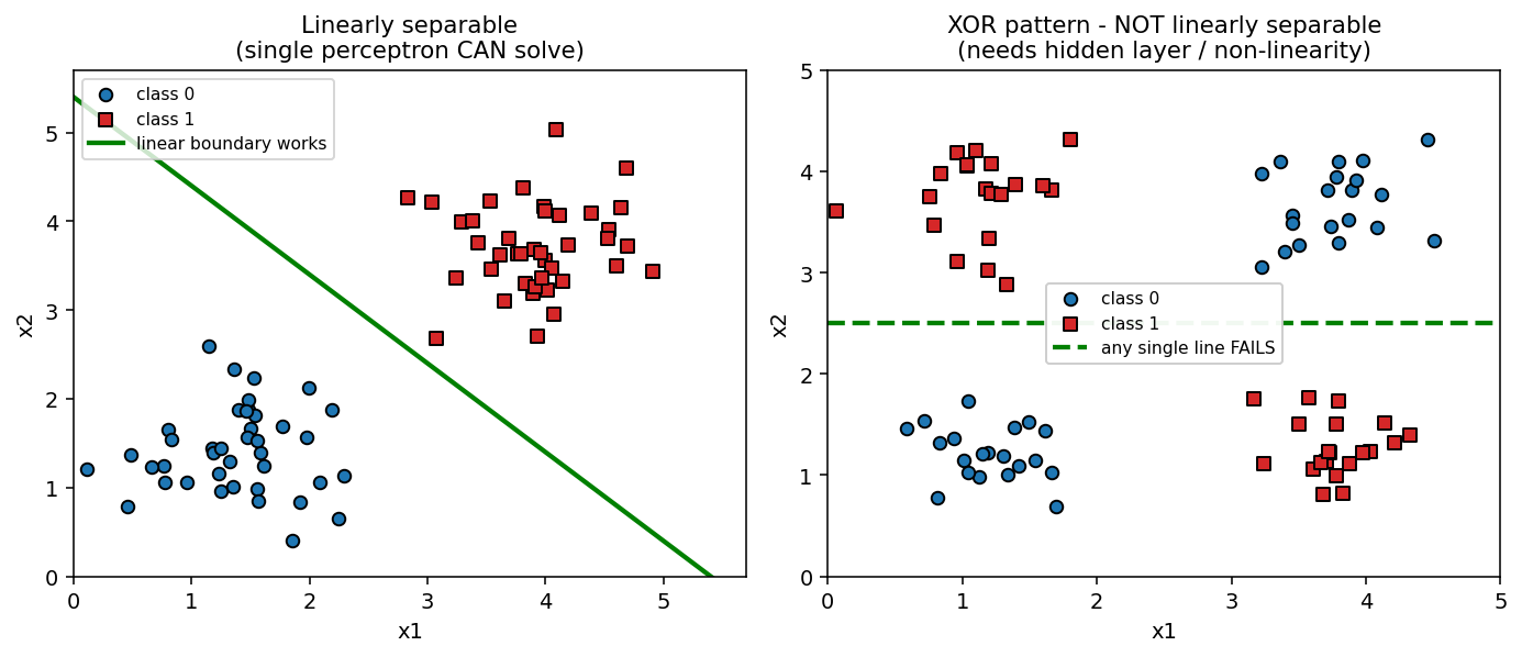
Figure 2 — Gradient descent on a loss surface.
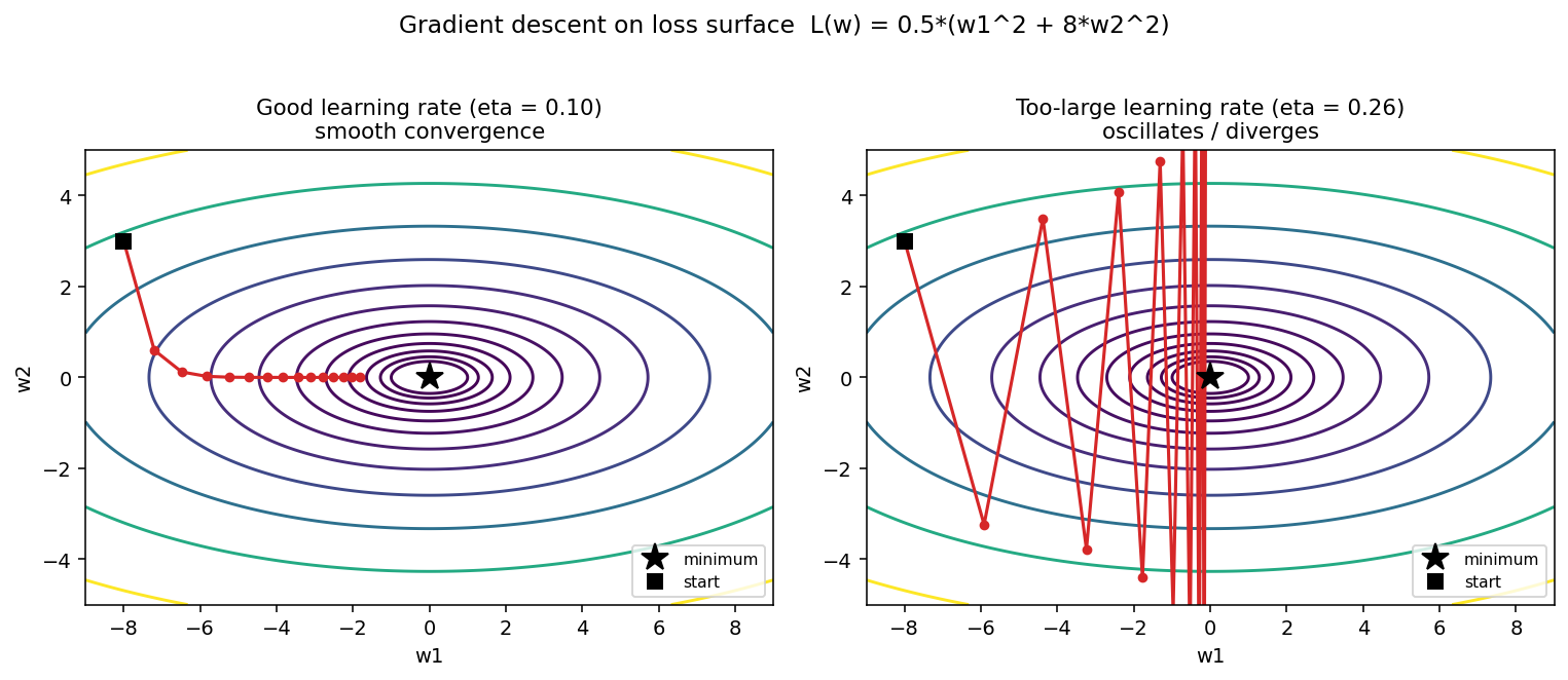
Figure 3 — Activation functions and their derivatives.
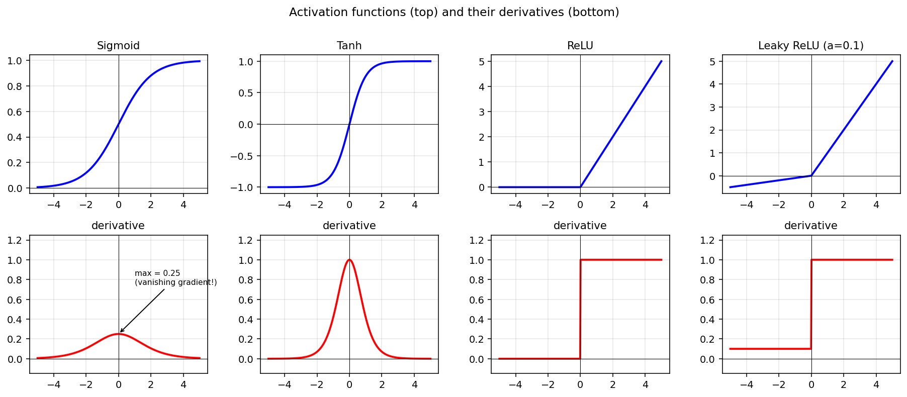
Figure 4 — Overfitting in the loss curves.
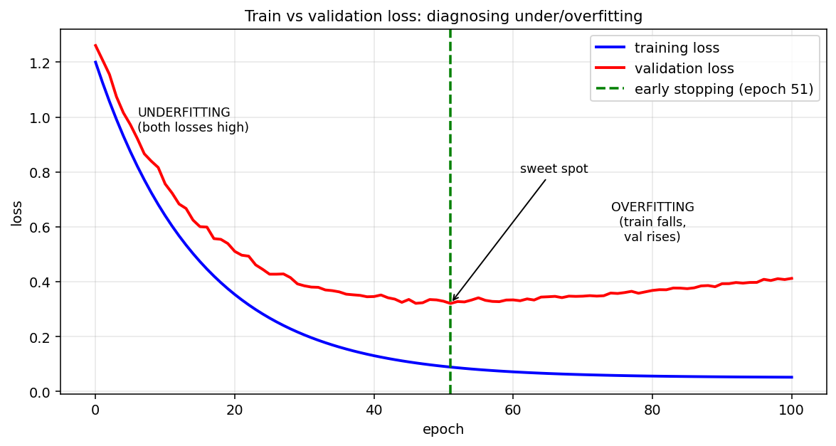
Figure 5 — Underfit / good fit / overfit on noisy 1-D data.
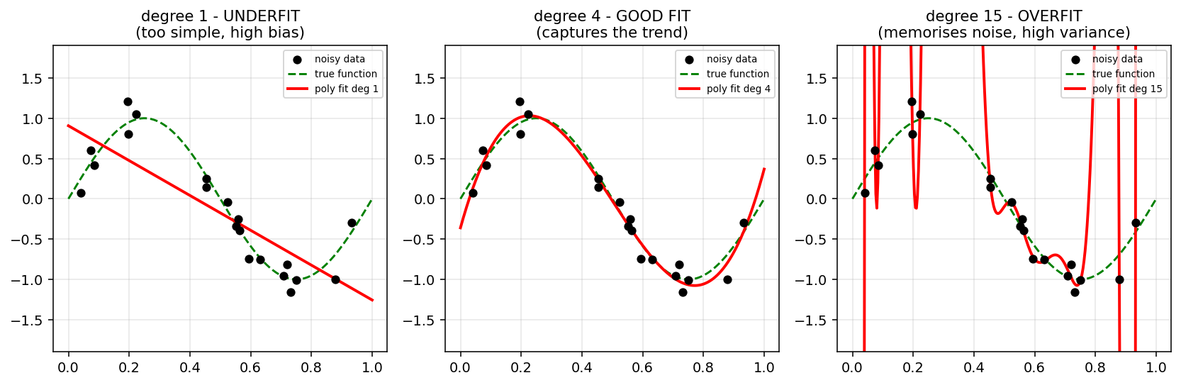
Figure 6 — Softmax in action.
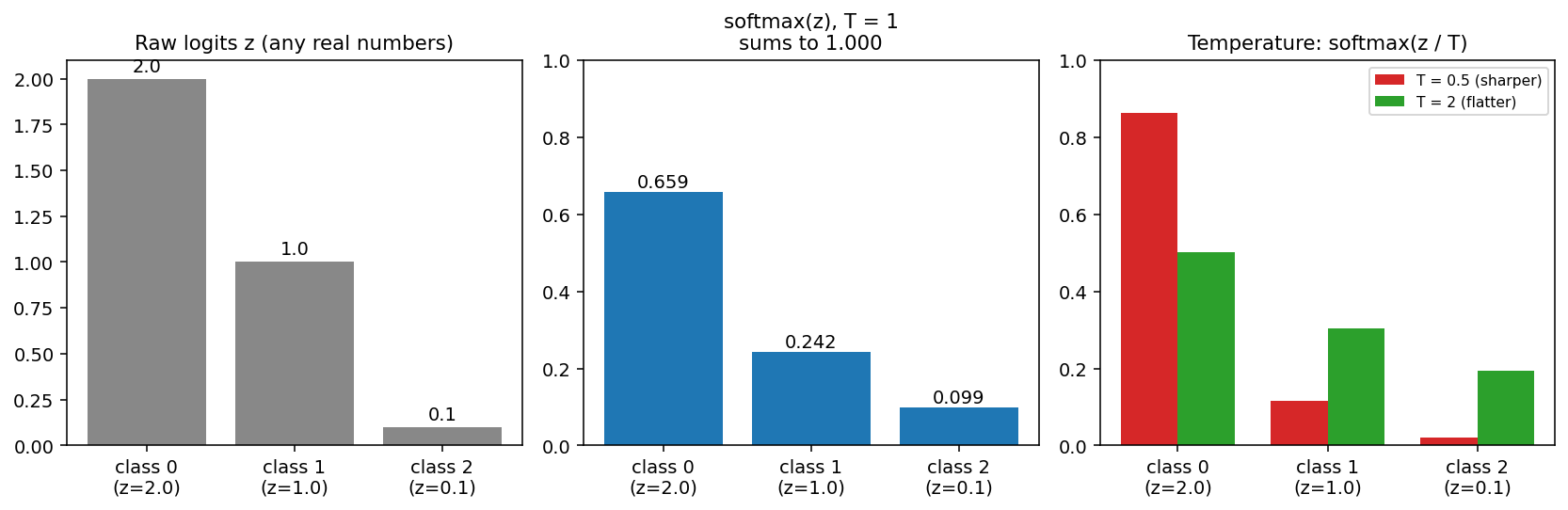
Figure 7 — k-NN decision regions, k = 1 vs k = 15.
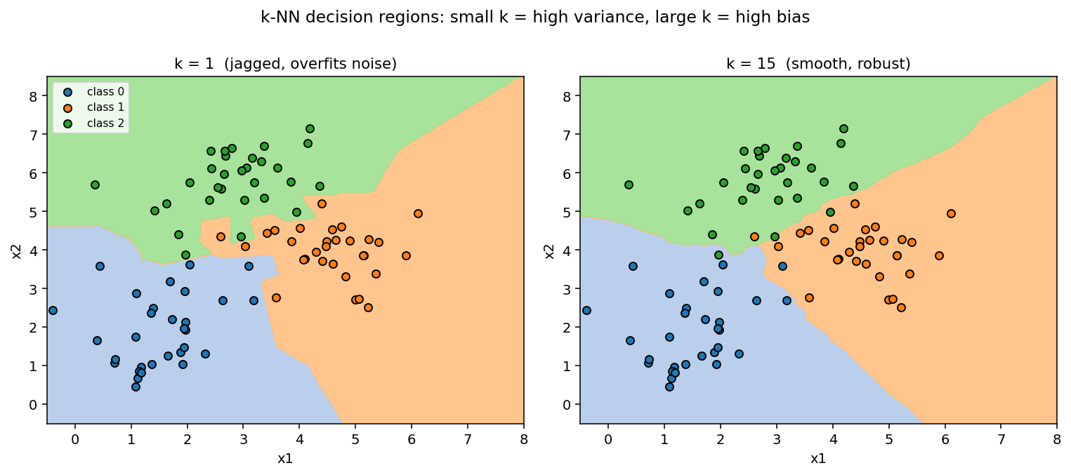
Figure 8 — CNN feature-map sizes through a tiny MNIST network.
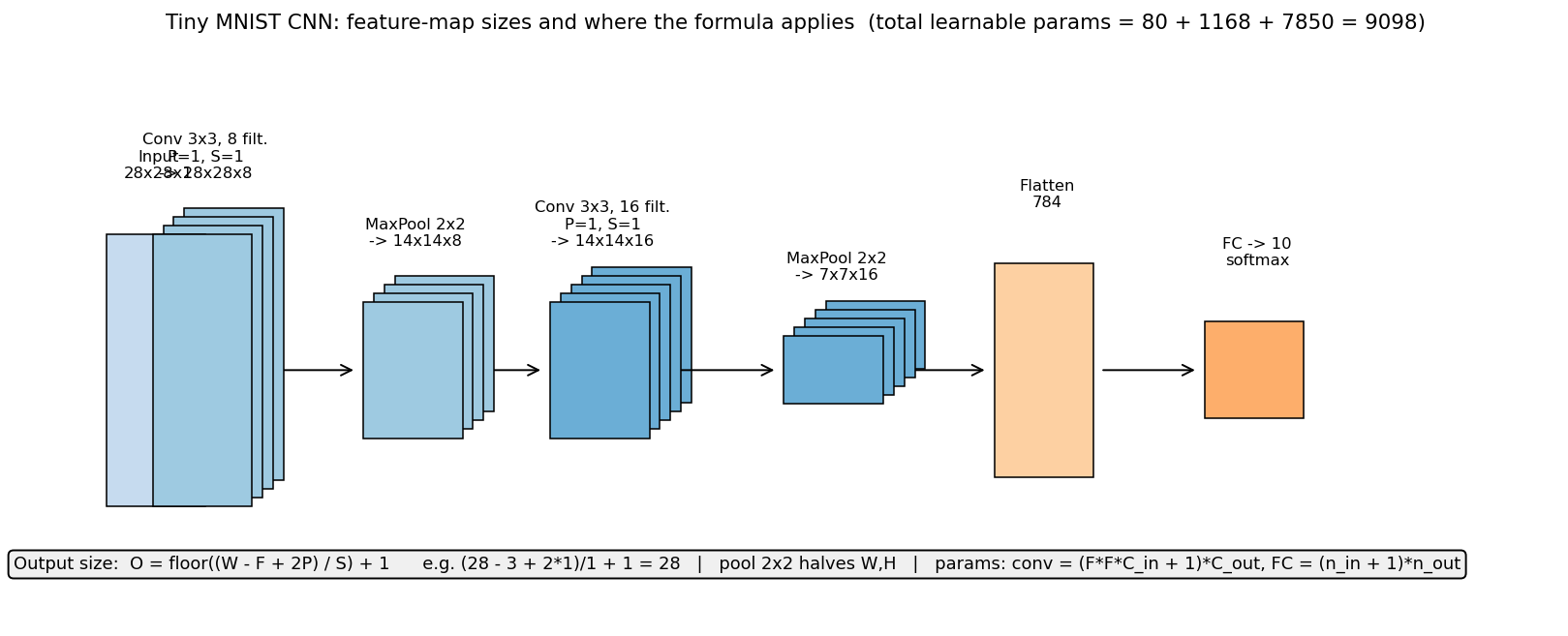
Figure 9 — Confusion-matrix heatmap (the trial-exam computation).
§6 Algorithms & Code¶
6.1 Gradient descent and backpropagation (pseudocode)¶
GRADIENT DESCENT                          BACKPROPAGATION (one batch)
1. initialize weights θ₀ randomly         1. forward pass: compute and STORE all
2. for t = 1 … T:                            intermediate activations and the loss L
     g_t = ∂L(θ_{t−1})/∂θ                 2. backward pass, output → input:
     θ_t = θ_{t−1} − η·g_t                     ∂L/∂W_l, ∂L/∂b_l, ∂L/∂x_l via chain rule,
3. return θ_T                                  reusing the stored forward values
                                           3. update every parameter: W ← W − η·∂L/∂W
বাংলা নোট: Backprop-এ "store" শব্দটা গুরুত্বপূর্ণ — forward pass-এর মাঝের মানগুলো না রাখলে backward pass-এ আবার সব হিসাব করতে হতো; জমিয়ে রাখার বিনিময়ে memory খরচ হয়, গতি বাড়ে।
6.2 Tiny perceptron from scratch (NumPy)¶
import numpy as np

class Perceptron:
    def __init__(self, n_features, lr=0.1):
        self.w = np.zeros(n_features); self.b = 0.0; self.lr = lr
    def predict(self, X):
        return (X @ self.w + self.b > 0).astype(int)
    def fit(self, X, y, epochs=20):
        for _ in range(epochs):
            for xi, yi in zip(X, y):
                pred = int(xi @ self.w + self.b > 0)
                err  = yi - pred                     # 0 if correct, ±1 if wrong
                self.w += self.lr * err * xi         # move boundary toward mistake
                self.b += self.lr * err
বাংলা নোট: ভুল হলেই (err = ±1) সীমানা-রেখাটা ভুল-করা point-এর দিকে একটু সরে — এটাই Rosenblatt-এর আদি শেখার নিয়ম; data linearly separable হলে এই loop নিশ্চিতভাবে থামে।
6.3 Softmax + cross-entropy from scratch (with the stability trick)¶
def softmax(z):                                  # z: (batch, K) logits
    z = z - z.max(axis=1, keepdims=True)         # shift invariance => no overflow
    e = np.exp(z)
    return e / e.sum(axis=1, keepdims=True)

def cross_entropy(probs, y_int):                 # y_int: integer labels
    return -np.log(probs[np.arange(len(y_int)), y_int]).mean()

def grad_logits(probs, y_int):                   # the famous p - y
    g = probs.copy()
    g[np.arange(len(y_int)), y_int] -= 1.0
    return g / len(y_int)
বাংলা নোট: প্রথম লাইনটাই §4.5-এর shift-invariance ধর্মের প্রয়োগ — max বিয়োগ করলে ফল অপরিবর্তিত কিন্তু \(e^z\) আর overflow করে না; আর শেষ function-টা §4.6-এর \(p - y\) সূত্র, এক লাইনে।
6.4 PyTorch MNIST classifier (exercise sheet 4, task 3)¶
import torch, torch.nn as nn, torch.nn.functional as F

class Network(nn.Module):
    def __init__(self):
        super().__init__()
        self.flatten = nn.Flatten()
        self.fc1 = nn.Linear(28*28, 128)         # (784+1)*128 = 100,480 params
        self.fc2 = nn.Linear(128, 10)            # (128+1)*10  =   1,290 params
    def forward(self, x):
        x = self.flatten(x)
        x = F.relu(self.fc1(x))
        return F.log_softmax(self.fc2(x), dim=1)

device  = torch.device('cuda' if torch.cuda.is_available() else 'cpu')
model   = Network().to(device)
opt     = torch.optim.Adam(model.parameters(), lr=1e-3)
loss_fn = nn.NLLLoss()                           # pairs with log_softmax

for epoch in range(5):                           # 5 epochs = 5 full passes
    model.train()
    for X, y in train_loader:                    # X already scaled to [0, 1]
        X, y = X.to(device), y.to(device)
        opt.zero_grad()                          # 1. clear old gradients
        loss = loss_fn(model(X), y)              # 2. forward + loss
        loss.backward()                          # 3. backprop (autograd)
        opt.step()                               # 4. gradient-descent update
Classic mistakes: forgetting opt.zero_grad() (gradients accumulate!); mixing \(\log _\operatorname{softmax}\) + nn.CrossEntropyLoss (double softmax — silent bug); forgetting model.train() / model.eval() around training/evaluation.
বাংলা নোট: Training loop-এর চার-তালের ছন্দ মুখস্থ করো: zero_grad → forward → backward → step। আর জোড়াগুলো মেলাও: \(\log _\operatorname{softmax}\) + NLLLoss, অথবা raw logits + CrossEntropyLoss — দুটো মেশালে নিঃশব্দে ভুল train হবে।
6.5 Confusion matrix + metrics from scratch¶
def confusion(y_true, y_pred, K):
    M = np.zeros((K, K), dtype=int)
    for t, p in zip(y_true, y_pred):
        M[t, p] += 1                                  # rows = actual, cols = predicted
    return M

def metrics(M):
    total = M.sum()
    acc   = np.trace(M) / total                       # diagonal sum / total
    sens  = M.diagonal() / M.sum(axis=1)              # per-class TP / (TP+FN)
    spec  = []
    for c in range(M.shape[0]):
        TP = M[c, c]
        FN = M[c, :].sum() - TP                       # rest of row c
        FP = M[:, c].sum() - TP                       # rest of column c
        TN = total - TP - FN - FP
        spec.append(TN / (TN + FP))
    return acc, sens, np.array(spec)
বাংলা নোট: এই কোডটা §4.13-এর সূত্রের হুবহু অনুবাদ — sensitivity আসে সারির যোগফল থেকে, specificity-র জন্য TN বের করতে হয় "মোট − TP − FN − FP" দিয়ে। Exam-এর হিসাব শেষে এই code-এ মিলিয়ে নিতে পারো।
6.6 k-fold cross-validation¶
def k_fold(model_fn, X, y, K=5):
    idx   = np.random.permutation(len(X))
    folds = np.array_split(idx, K)
    scores = []
    for k in range(K):
        val_idx   = folds[k]
        train_idx = np.concatenate([folds[i] for i in range(K) if i != k])
        m = model_fn().fit(X[train_idx], y[train_idx])
        scores.append(m.score(X[val_idx], y[val_idx]))
    return np.mean(scores), np.std(scores)
বাংলা নোট: প্রতিটা fold ঠিক একবার validation হয় — তাই ফলাফল কোনো একটা "ভাগ্যবান split"-এর ওপর নির্ভর করে না; std-টাও report করো, সেটা estimate-এর অনিশ্চয়তা বলে দেয়।
6.7 Pretrained object detection (exercise sheet 4, task 4)¶
import torch, torchvision

model = torchvision.models.detection.fasterrcnn_mobilenet_v3_large_fpn(
            weights="DEFAULT").eval()
img = torchvision.io.read_image("dog.jpg") / 255.0       # float in [0, 1]
with torch.no_grad():
    out = model([img])
keep   = out[0]['scores'] > 0.3                          # confidence filter
boxes  = out[0]['boxes'][keep]
labels = out[0]['labels'][keep]
# draw boxes ...
Why pretrained? Transfer learning: the backbone already learned generic visual features on huge datasets — you save data, compute, and time. (Exactly the lecture's advice: "Can you use transfer learning to reduce the amount of data you need?")
বাংলা নোট: শূন্য থেকে detector train করতে লাখো labelled ছবি লাগে; pretrained model-এর backbone আগেই সাধারণ visual feature শিখে রেখেছে — তাই অল্প data-তেও কাজ চলে। Score > 0.3 filter-টা কম-আত্মবিশ্বাসী detection ছেঁটে ফেলে।
§7 Trial-Exam Mapping¶
| Trial-exam question | What it asks | Where in this chapter |
|---|---|---|
| Q3a-i | Compute accuracy from a 3×3 confusion matrix | §4.13 formulas + worked example, Figure 9, code §6.5 |
| Q3a-ii | Compute specificity for class 2 | §4.13 (TN/(TN+FP), with TN = total − TP − FN − FP) |
| Q3a-iii | Find the class with the highest sensitivity | §4.13 (per-class TP / row-sum, then compare) |
| Q3b | Define an epoch | §2.9 — "one complete pass of the entire training dataset through the network" |
| Q3c-1 (T/F) | "To choose the best hyperparameters, divide data into training, validation and test data" | TRUE — §2.10/§4.9: validation selects hyperparameters, test stays untouched |
| Q3c-2 (T/F) | "The data should be normalized after splitting into training and test data" | TRUE — §4.9: statistics from the training split only; otherwise leakage |
| Q3c-3 (T/F) | "To avoid overfitting, it is always better to add more layers" | FALSE — §2.4/§2.11: more layers → more parameters → more overfitting risk + vanishing gradients |
বাংলা: Trial exam-এর Chapter-4 অংশের পুরো ১০ নম্বরই উপরের টেবিলে — confusion matrix-এর তিনটা হিসাব (সবচেয়ে বেশি নম্বর, §4.13 মুখস্থ-সমান করে রাখো), epoch-এর এক-লাইনের definition, আর তিনটা True/False যার উত্তর: সত্য, সত্য, মিথ্যা। শেষেরটা মনে রাখার কৌশল: "always better" জাতীয় চরম দাবি প্রায় সবসময় মিথ্যা।
§8 Mock Exam — 20 Questions (4 Tiers × 5)¶
Attempt everything on paper before opening the solutions. Tier A ≈ warm-up definitions, Tier B ≈ intuition/explanation, Tier C ≈ full hand computations (trial-exam style and harder), Tier D ≈ transfer questions slightly beyond the lecture — exactly the kind a professor uses to separate grades.
Tier A — Basic (5 questions)¶
A1. Define precisely: (a) epoch, (b) batch size, © learning rate. For a training set of 10,000 samples and batch size 50, how many weight updates happen in 3 epochs?
A2. What is the difference between supervised and unsupervised learning? Give one computer-vision example of each. Is "predicting a house price from census features" classification or regression?
A3. Write down the softmax function for logits \(z = (z_{1}, \ldots , z_{K})\) and state two of its mathematical properties.
A4. Name the three dataset splits and the exact role of each. Why must normalization statistics be computed after splitting?
A5. For a binary confusion matrix with entries TP, FP, FN, TN, write the formulas for accuracy, sensitivity, specificity and prevalence.
Tier B — Intuitive (5 questions)¶
B1. Why can a single perceptron not solve the XOR problem, and what two ingredients does a network need to solve it? (Refer to Figure 1.)
B2. Explain gradient descent with the hiker-in-fog analogy, then describe what goes wrong when the learning rate is (a) much too large and (b) much too small. (Refer to Figure 2.)
B3. A COVID test has 99 % sensitivity and 99 % specificity. In a population of 10,000 with 1 % prevalence, show with numbers why a positive result is only 50 % trustworthy, while accuracy is still 99 %.
B4. Give two reasons why convolution layers (weight sharing + local windows) beat fully-connected layers on images. Support one reason with a rough parameter count for a 1000×1000 grayscale input.
B5. During training you observe: training loss steadily decreasing, validation loss decreasing for 30 epochs and then steadily rising. Diagnose the situation and name three different remedies.
Tier C — Harder, compute by hand (5 questions)¶
C1. Model \(\hat{y} = w\cdot x + b\), data {(1, 3), (2, 5)}, current \(w = 0.5, b = 0.5\), learning rate \(\eta = 0.05\), loss = MSE. Compute: the current loss, both gradients, the updated parameters, and the new loss (show that it decreased).
C2. Backpropagate the 2-layer ReLU network \(h = ReLU(w_{1}x + b_{1})\), \(\hat{y} = w_{2}h + b_{2}\), \(L = \tfrac{1}{2}(\hat{y} - y)^{2}\) at \(x = 1, y = 2\), with \(w_{1} = 1, b_{1} = 0, w_{2} = 1, b_{2} = 0\). Compute the forward pass, all four gradients, the updated parameters for \(\eta = 0.1\), and the new loss.
C3. A CNN receives a 32×32×3 image: conv layer 1 = 8 filters of 5×5, stride 1, no padding; then 2×2 max-pool; conv layer 2 = 16 filters of 3×3, stride 1, padding 1; then flatten and a dense layer to 10 outputs. Give every intermediate tensor shape and the parameter count of each learnable layer, plus the total.
C4. For the confusion matrix below (rows = actual, columns = predicted), compute the overall accuracy, the specificity of class 1, and identify the class with the highest sensitivity.
C5. Logits \(z = (3, 1, 0)\), true class = class 1 (one-hot \(y = (1, 0, 0)\)). Compute the softmax probabilities, the cross-entropy loss, and the gradient \(\partial L/\partial z\). (Use e³ ≈ 20.09, e¹ ≈ 2.718, e⁰ = 1.)
Tier D — Transfer, beyond the lecture (5 questions)¶
D1. The lecture used sigmoid activations. Show quantitatively why a deep stack of sigmoid layers suffers from vanishing gradients (use the bound on σ′), and explain how ReLU fixes it. What new problem can ReLU introduce, and which variant addresses that?
D2. The lecture introduced MSE for regression. Why is cross-entropy preferred over MSE for classification with a softmax (or sigmoid) output? Argue with the gradient: what factor appears in the MSE+sigmoid gradient that disappears with cross-entropy?
D3. Define temperature-scaled softmax \(\operatorname{softmax}(z/T)\). For \(z = (2.0, 1.0, 0.1)\), the probabilities at T = 1 are (0.659, 0.242, 0.099). Compute (or closely estimate) the winning-class probability at T = 0.5 and at T = 2, and state the limiting behaviour as T → 0 and T → ∞. Name one practical use of temperature.
D4. Compare L2 and L1 regularization: write both penalties, derive what each does inside the gradient-descent update, and explain geometrically why L1 produces sparse weights while L2 only shrinks them.
D5. Batch normalization was not covered in the lecture. Write its transformation (training time), explain what γ and β are for, and give two reasons it helps training deep networks. What changes at test time?
§8.5 Solutions¶
Tier A solutions¶
A1. (a) Epoch = one complete pass of the entire training dataset through the network — every training sample has contributed to gradient updates exactly once. (b) Batch size = the number of samples processed before one weight update is performed. © Learning rate = the step-size factor η multiplying the negative gradient in each update \(w \leftarrow w - \eta \cdot \partial L/\partial w\). Updates: per epoch \(10000/50 = 200\) updates; in 3 epochs \(3 \times 200 = 600\) weight updates. বাংলা: Epoch-এর এক লাইনের সংজ্ঞাটাই trial exam-এ সরাসরি এসেছে — পুরো training data-র একটি সম্পূর্ণ pass; আর update সংখ্যা = epoch × (N/B)।
A2. Supervised: every training input comes with a desired output (label); the model learns the input→output map. Example: digit classification on MNIST (labelled images). Unsupervised: no labels; the algorithm finds structure on its own. Example: clustering image patches / autoencoder compression of images. House-price prediction outputs a continuous number → regression (supervised). বাংলা: Label থাকলে supervised, না থাকলে unsupervised; আর output সংখ্যা হলে regression, class হলে classification — এই দুই প্রশ্ন এক সাথেই মনে রাখো।
A3.
Any two of: (1) every output lies in (0, 1); (2) outputs sum to exactly 1 (valid probability distribution); (3) order-preserving — the largest logit gets the largest probability; (4) invariant to adding a constant c to all logits, since e^c cancels in numerator and denominator (used for numerical stability via \(z - \max (z)\)). বাংলা: Softmax logit-কে probability বানায়; পরীক্ষায় property লিখতে বললে "যোগফল 1" আর "ধ্রুবক যোগে অপরিবর্তিত (প্রমাণ: e^c কাটাকাটি)" — এই দুটোই সবচেয়ে দামি।
A4. Training set: fits the weights via gradient descent. Validation set: compares hyperparameter choices (architecture, η, epochs) and triggers early stopping. Test set: used exactly once at the very end for the unbiased final score. Normalization after splitting: the mean/min/max must come from the training data only; if computed on the full dataset, information about the test distribution leaks into training and the test score becomes optimistically biased. বাংলা: তিন set-এর তিন কাজ: শেখা / বাছাই / চূড়ান্ত রায়; আর normalization-এর পরিসংখ্যান শুধু train থেকে — নইলে data leakage।
A5.
Accuracy    = (TP + TN) / (TP + TN + FP + FN)
Sensitivity = TP / (TP + FN)
Specificity = TN / (TN + FP)
Prevalence  = (TP + FN) / (TP + TN + FP + FN)
বাংলা: Sensitivity-র হর হলো "আসল positive-রা" (TP+FN), specificity-র হর "আসল negative-রা" (TN+FP) — হর গুলিয়ে ফেলাই সবচেয়ে কমন ভুল।
Tier B solutions¶
B1. A single perceptron computes \(a(w\cdot x + b)\): its decision boundary is the straight line/hyperplane \(w\cdot x + b = 0\). In XOR, the two classes sit on the two diagonals of a square — any straight line that separates one diagonal pair necessarily misclassifies at least one point of the other pair (no line can have both blue corners on one side and both red corners on the other). The fix needs (1) at least one hidden layer (so the input space is first re-mapped) and (2) a non-linear activation (otherwise stacked linear layers collapse into one linear map and the boundary is still a line). With both, a 2-2-1 network solves XOR easily. বাংলা: এক perceptron = এক সরলরেখা, আর XOR-এর কোণাকুণি class কোনো সরলরেখায় ভাগ হয় না; hidden layer + non-linearity — দুটোই লাগবে, একটাও বাদ দিলে চলবে না।
B2. Hiker in fog: the loss surface is a foggy mountain landscape; you only feel the local slope (gradient) and repeatedly step downhill (negative gradient) with step length η. (a) η much too large: each step overshoots the valley floor and lands on the opposite slope, possibly higher than before — the iterates oscillate or diverge (Figure 2, right). (b) η much too small: every step is microscopic — convergence is guaranteed on nice surfaces but takes absurdly many steps, and you can stall in flat regions / get stuck near shallow local minima. বাংলা: η বড় → উপত্যকা টপকে ওপারে, লাফাতে লাফাতে diverge; η ছোট → পৌঁছাবে, কিন্তু পিঁপড়ার গতিতে — মাঝামাঝি একটা ভালো η-ই শিল্প।
B3. Population 10,000, prevalence 1 % → 100 infected, 9,900 healthy. Sensitivity 99 %: TP = 99, FN = 1. Specificity 99 %: TN = 0.99·9900 = 9801, FP = 99. Accuracy = (99 + 9801)/10000 = 9900/10000 = 99 %. But among positive results: positives reported = TP + FP = 99 + 99 = 198, of which truly sick = 99 → P(sick | positive) = 99/198 = 50 %. The healthy group is so large that its 1 % error rate produces as many false positives as there are true positives. (Negative results are fine: P(healthy | negative) = 9801/9802 ≈ 99.99 %.) বাংলা: Prevalence কম হলে সুস্থদের সামান্য ভুলও সংখ্যায় রোগীদের সমান হয়ে যায় — তাই ৯৯% accuracy সত্ত্বেও positive মানে আধাআধি সংশয়; এটাই "fallacy of accurate tests"।
B4. Reason 1 — parameter explosion: one fully-connected hidden layer with just 1000 neurons on a 1000×1000 = 10⁶-pixel input needs ≈ 10⁶ × 10³ = 10⁹ weights; a conv layer with 32 filters of 3×3 needs (3·3·1+1)·32 = 320 parameters, independent of image size. Reason 2 — built-in structure: the same kernel applied everywhere (weight sharing) means a pattern learned at one location is recognized at every location (translation robustness), and local windows match the local nature of image statistics (edges, textures). Fully-connected layers must relearn each pattern at each position and can permute pixels without noticing. বাংলা: Conv layer-এর parameter ছবির আকারে বাড়ে না (weight sharing), আর এক জায়গায় শেখা pattern সব জায়গায় চেনে — ছবির জন্য এই দুই গুণই FC layer-এর কাছে নেই।
B5. Diagnosis: classic overfitting starting near epoch 30 — the model keeps improving on memorised training data while generalisation worsens. Remedies (any three): early stopping at the validation minimum; stronger regularization (L2 weight decay, dropout); data augmentation / collect more data; reduce model capacity (fewer layers/neurons); batch normalization; k-fold to verify. Not a remedy: training longer or adding layers — both worsen it. বাংলা: Validation loss-এর ঘুরে দাঁড়ানোই overfitting-এর স্বাক্ষর; দাওয়াই — আগেভাগে থামা, regularize করা, data বাড়ানো; আর "আরো layer" হলো উল্টো বিষ।
Tier C solutions¶
C1.
Forward:   ŷ⁽¹⁾ = 0.5·1 + 0.5 = 1.0    r₁ = 1.0 − 3 = −2.0
           ŷ⁽²⁾ = 0.5·2 + 0.5 = 1.5    r₂ = 1.5 − 5 = −3.5
Loss:      E = (1/2)( 4 + 12.25 ) = 8.125

Gradients: ∂E/∂w = (2/2)( (−2.0)·1 + (−3.5)·2 ) = −2 − 7 = −9
           ∂E/∂b = (2/2)( −2.0 − 3.5 )           = −5.5

Update:    w ← 0.5 − 0.05·(−9)   = 0.5 + 0.45  = 0.95
           b ← 0.5 − 0.05·(−5.5) = 0.5 + 0.275 = 0.775

Verify:    ŷ⁽¹⁾ = 0.95 + 0.775 = 1.725   r₁ = −1.275
           ŷ⁽²⁾ = 1.9 + 0.775  = 2.675   r₂ = −2.325
           E_new = (1.6256 + 5.4056)/2 = 3.516  <  8.125  ✓ decreased
বাংলা: ছন্দটা সবসময় এক: forward → residual → gradient (residual×input-এর গড়ের দ্বিগুণ) → update → আবার forward দিয়ে যাচাই। যাচাইয়ের লাইনটাই নম্বর বাঁচায়।
C2.
Forward:   z₁ = 1·1 + 0 = 1     h = ReLU(1) = 1
           ŷ  = 1·1 + 0 = 1     L = ½(1 − 2)² = 0.5

Backward:  ∂L/∂ŷ  = ŷ − y = −1
           ∂L/∂w₂ = (−1)·h = −1          ∂L/∂b₂ = −1
           ∂L/∂h  = (−1)·w₂ = −1
           ReLU′(z₁) = 1  (since z₁ = 1 > 0)   →  ∂L/∂z₁ = −1
           ∂L/∂w₁ = (−1)·x = −1          ∂L/∂b₁ = −1

Update (η = 0.1):  w₁ = 1.1,  b₁ = 0.1,  w₂ = 1.1,  b₂ = 0.1

Verify:    z₁ = 1.1 + 0.1 = 1.2    h = 1.2
           ŷ  = 1.1·1.2 + 0.1 = 1.42
           L  = ½(1.42 − 2)² = ½·(0.58)² = 0.168  <  0.5  ✓
বাংলা: ReLU-র local gradient হয় 1 নয়তো 0 — এখানে z₁ > 0 তাই gradient অবাধে পেছনে গেছে; z₁ ঋণাত্মক হলে চারটা gradient-এর দুটো (w₁, b₁) শূন্য হয়ে যেত — এটাই "dead ReLU"-র এক ঝলক।
C3.
Input:                          32×32×3
conv1 (8 @ 5×5, S=1, P=0):      O = (32−5+0)/1 + 1 = 28      → 28×28×8
        params = (5·5·3 + 1)·8 = 76·8 = 608
pool1 (2×2, S=2):               → 14×14×8                      params = 0
conv2 (16 @ 3×3, S=1, P=1):     O = (14−3+2)/1 + 1 = 14      → 14×14×16
        params = (3·3·8 + 1)·16 = 73·16 = 1168
flatten:                        14·14·16 = 3136
dense (3136 → 10):              params = (3136 + 1)·10 = 31,370

TOTAL = 608 + 1168 + 31,370 = 33,146 parameters
বাংলা: দুটো ফাঁদ খেয়াল করো: filter-এর গভীরতা সবসময় আগের layer-এর channel সংখ্যা (প্রথমে 3, পরে 8), আর শেষের dense layer-ই মোট parameter-এর সিংহভাগ খেয়ে নেয় — CNN-এ প্রায়ই এমন হয়।
C4.
Total = 60.    Diagonal = 15 + 16 + 15 = 46.
Accuracy = 46/60 ≈ 0.767  (76.7 %)

Specificity of class 1:
  TP₁ = 16
  FN₁ = 2 + 2 = 4              (rest of row 1)
  FP₁ = 3 + 4 = 7              (rest of column 1)
  TN₁ = 60 − 16 − 4 − 7 = 33
  Specificity₁ = 33/(33 + 7) = 33/40 = 0.825

Sensitivities:  class 0: 15/20 = 0.75
                class 1: 16/20 = 0.80   ← highest
                class 2: 15/20 = 0.75
বাংলা: Row-sum গুলো এখানে সব ২০ — তাই sensitivity তুলনা মানে স্রেফ diagonal তুলনা; specificity-তে TN বের করার সূত্র "মোট − TP − FN − FP" ভুলো না।
C5.
e³ = 20.09,  e¹ = 2.718,  e⁰ = 1        Σ = 23.81
p = (20.09/23.81, 2.718/23.81, 1/23.81) = (0.844, 0.114, 0.042)     (sums to 1 ✓)

Cross-entropy:  L = −ln(p₁) = −ln(0.844) = 0.170

Gradient:       ∂L/∂z = p − y = (0.844 − 1, 0.114, 0.042)
                       = (−0.156, 0.114, 0.042)
বাংলা: সঠিক class-এর gradient ঋণাত্মক (logit বাড়াও), ভুল class-দের ধনাত্মক (কমাও), আর তিনটা component-এর যোগফল শূন্য — \(p - y\)-এর এই তিন চিহ্নই উত্তর যাচাইয়ের যন্ত্র।
Tier D solutions¶
D1. The sigmoid derivative satisfies \(\sigma '(x) = \sigma (x)(1 - \sigma (x)) \le 0.25\), with equality only at x = 0, and \(\sigma ' \approx 0\) for |x| > 4 (saturation). Backprop through n sigmoid layers multiplies the upstream gradient by one σ′ factor per layer, so its magnitude is bounded by \(0.25^{n}\): for n = 10, \(0.25^{10} \approx 9.5\cdot 10^{-7}\) — early layers receive a learning signal a million times weaker and effectively stop learning. ReLU's derivative is exactly 1 for all positive inputs, so gradients pass through active units unattenuated, no matter the depth; it is also cheap (a comparison) and creates sparse activations. New problem: dying ReLU — a unit pushed into the negative regime has derivative 0 forever and can never recover. Fix: leaky ReLU \(\max (\alpha x, x)\) with small α (e.g. 0.01–0.1), which keeps a nonzero gradient on the negative side (also ELU/GELU). বাংলা: σ′ ≤ 0.25, আর দশ layer মানে 0.25¹⁰ ≈ ১০⁻⁶ গুণ দুর্বল সংকেত — সামনের layer শেখাই বন্ধ করে দেয়; ReLU-র ঢাল ধনাত্মক দিকে পুরো ১ বলে গভীরতাতেও সংকেত বাঁচে, আর তার "মৃত neuron" রোগের টিকা হলো leaky ReLU।
D2. With sigmoid output \(p = \sigma (z)\) and MSE loss \(L = \tfrac{1}{2}(p - y)^{2}\), the chain rule gives \(\partial L/\partial z = (p - y)\cdot \sigma '(z)\). The factor σ′(z) is the killer: if the model is confidently wrong (e.g. y = 1 but z ≪ 0 so p ≈ 0), σ′(z) ≈ 0 and the gradient vanishes exactly when the strongest correction is needed — learning stalls. With cross-entropy \(L = -[y\cdot \ln p + (1-y)\cdot \ln (1-p)]\), the σ′ factor cancels against the 1/(p(1−p)) from the log derivative, leaving \(\partial L/\partial z = p - y\): large error → large gradient, always. Same story for softmax + categorical cross-entropy (\(\partial L/\partial z = p - y\), §4.6). Additionally, cross-entropy is the maximum-likelihood objective for a Bernoulli/categorical output model, while MSE corresponds to a Gaussian assumption that is wrong for probabilities. বাংলা: MSE+sigmoid-এর gradient-এ σ′ গুণক থাকে — model যত আত্মবিশ্বাসী-ভুল, gradient তত মৃত; cross-entropy-তে σ′ কেটে গিয়ে থাকে নিখাদ \(p - y\) — ভুল বড় হলে ধাক্কাও বড়, তাই classification-এ cross-entropy-ই সঠিক জুটি।
D3.
softmax_T(z)ᵢ = e^(zᵢ/T) / Σⱼ e^(zⱼ/T)

T = 0.5:  z/T = (4, 2, 0.2)
          e⁴ = 54.60, e² = 7.389, e^0.2 = 1.221    Σ = 63.21
          p = (0.864, 0.117, 0.019)        → winner sharpened 0.659 → 0.864
T = 2:    z/T = (1, 0.5, 0.05)
          e¹ = 2.718, e^0.5 = 1.649, e^0.05 = 1.051    Σ = 5.418
          p = (0.502, 0.304, 0.194)        → flattened 0.659 → 0.502
Limits: T → 0⁺ → one-hot on the argmax (hard max); T → ∞ → uniform distribution 1/K. Practical uses: knowledge distillation (a high T exposes the teacher's "dark knowledge" in the small probabilities), sampling diversity control in generative models, confidence calibration. বাংলা: T ছোট → বণ্টন তীক্ষ্ণ, বিজয়ীই সব; T বড় → বণ্টন চ্যাপ্টা, সবাই কাছাকাছি; T-এর দুই সীমা হলো argmax আর uniform — distillation-এ বড় T দিয়েই শিক্ষক-model-এর লুকানো জ্ঞান ছাত্রকে দেখানো হয়।
D4.
L2:  penalty (λ/2)·Σ wᵢ²    gradient λ·w        update  w ← (1 − ηλ)·w − η·∂L_data/∂w
L1:  penalty λ·Σ |wᵢ|       gradient λ·sign(w)  update  w ← w − ηλ·sign(w) − η·∂L_data/∂w
L2 shrinks each weight by a proportional factor (1 − ηλ) — big weights shrink a lot, small weights barely move, and nothing reaches exactly 0. L1 subtracts a constant ηλ each step regardless of magnitude — small weights are driven exactly to 0 and stay there → sparsity (automatic feature selection). Geometry: minimizing the data loss subject to a penalty budget means finding where the loss contours (ellipses) first touch the constraint region. The L2 region \(\Sigma w_{i}^{2} \le t\) is a smooth ball — the touching point is generically off-axis (all coordinates nonzero, just small). The L1 region \(\Sigma |w_{i}| \le t\) is a diamond (cross-polytope) whose sharp corners lie on the coordinate axes — contours overwhelmingly touch first at a corner, where some coordinates are exactly 0. বাংলা: L2 প্রতিটা weight-কে আনুপাতিক হারে ছোট করে (শূন্য করে না), L1 প্রতি ধাপে ধ্রুবক পরিমাণ কাটে বলে ছোট weight ঠিক শূন্যে পৌঁছে যায়; জ্যামিতিতে — L2-এর গোল বলের গায়ে ellipse ছোঁয় যেখানে-সেখানে, কিন্তু L1-এর হীরার ধারালো কোণাগুলো অক্ষের ওপর বলে ছোঁয়া লাগে কোণাতেই — তাই sparsity।
D5.
For each unit, over a mini-batch B:
  μ_B = (1/|B|) Σ x           σ²_B = (1/|B|) Σ (x − μ_B)²
  x̂  = (x − μ_B) / √(σ²_B + ε)                (normalize: mean 0, variance 1)
  y   = γ·x̂ + β                               (learned scale γ and shift β)
γ and β are learned parameters that restore representational power: if the network prefers un-normalized activations, it can learn γ = √(σ²_B), β = μ_B and undo the normalization — so BN never reduces what the layer can express. Why it helps (any two): (1) keeps each layer's input distribution stable while earlier layers change ("internal covariate shift" reduction / a much smoother optimization landscape), allowing much larger learning rates; (2) gradients are insensitive to the scale of weights → less vanishing/exploding; (3) the batch noise in μ_B, σ²_B acts as a mild regularizer; (4) makes initialization less critical. At test time there is no batch: use running averages of μ and σ² accumulated during training (and the transformation becomes a fixed affine map that can be folded into the previous layer). বাংলা: BatchNorm প্রতি mini-batch-এ activation-কে mean-0/var-1 বানিয়ে তারপর শেখা γ, β দিয়ে আবার মাপ-মতো সাজায় — ফলে গভীর network-এও প্রতিটা layer স্থির বণ্টনের input পায়, বড় learning rate চলে, আর batch-এর কোলাহল ফাউ regularization দেয়; test-এ batch নেই বলে training-এ জমানো running average ব্যবহার হয়।
§9 Exam-Day Cheat Sheet¶
The eight formulas (write these from memory the night before):
1. Linear layer:      ŷ = W·x + b                      W: m×n, params = m·(n+1)
2. MSE + gradients:   E = (1/N)Σ(ŷ−y)²;   ∂E/∂w = (2/N)Σ(ŷ−y)·x;   ∂E/∂b = (2/N)Σ(ŷ−y)
3. Sigmoid:           σ(x) = 1/(1+e⁻ˣ);    σ′ = σ(1−σ) ≤ 0.25
4. Softmax:           pᵢ = e^(zᵢ)/Σⱼe^(zⱼ);  sums to 1;  shift-invariant (e^c cancels)
5. Cross-entropy:     L = −ln(p_true);      with softmax:  ∂L/∂z = p − y
6. Gradient descent:  w ← w − η·∂L/∂w       (L2 reg: w ← (1−ηλ)·w − η·∂L/∂w)
7. Conv output:       O = ⌊(W − F + 2P)/S⌋ + 1;   conv params = (F·F·C_in + 1)·C_out
8. Confusion matrix:  Acc = diag/total;  Sens = TP/(TP+FN);  Spec = TN/(TN+FP);
                      Prev = (TP+FN)/total;  TN_c = total − TP_c − FN_c − FP_c
Definition bullets (one line each): * Epoch = one full pass over the entire training set (N/B updates). * Validation set chooses hyperparameters; test set is touched once. * Normalize AFTER splitting, with training-set statistics only. * Overfitting = train loss falls while validation loss rises; fight with data, augmentation, dropout, L2, early stopping — never with "more layers". * k-NN: no training, majority vote of k nearest; small k overfits, large k underfits. * CNN: weight sharing + local kernels; conv extracts, pooling halves; pooling has 0 parameters. * Sigmoid saturates → vanishing gradient; ReLU derivative = 1 keeps gradients alive. * 99 %-accurate test at 1 % prevalence → a positive is right only 50 % of the time.
Hand-computation checklist (Tier C insurance): 1. Write the forward pass and store every intermediate value. 2. Differentiate outermost-first; each backward step multiplies one local derivative. 3. Update with the minus sign: \(\theta - \eta \cdot grad\). 4. Re-run the forward pass — the loss MUST have dropped; if not, recheck signs. 5. Confusion matrix: diagonal first, then row-rest = FN, column-rest = FP.
বাংলা মন্ত্র (পরীক্ষার ঠিক আগের ৬০ সেকেন্ড): * "Epoch মানে পুরো data একবার" — Q3b-র পুরো নম্বর এই এক বাক্যে। * "Sensitivity = রোগী ধরা, Specificity = সুস্থ চেনা" — হর যথাক্রমে (TP+FN) আর (TN+FP)। * "ভাগ আগে, normalize পরে" — train-এর পরিসংখ্যান দিয়েই সবাইকে রূপান্তর। * "বেশি layer ≠ ভালো" — overfitting আর vanishing gradient দুটোই বাড়ে; True/False-এ চোখ বন্ধ করে FALSE। * "Softmax-এ ধ্রুবক যোগে কিছু হয় না, cross-entropy-র gradient হলো p − y" — দুই লাইনেই Tier-D জেতা যায়। * "Update মানে minus eta gradient" — চিহ্ন ভুল মানে পাহাড়ে ওঠা, নামা নয়। * "O = (W − F + 2P)/S + 1, আর pooling-এর parameter শূন্য" — CNN-এর সব হিসাবের চাবি। * শান্ত থাকো: হিসাব শেষে সবসময় এক লাইনে যাচাই করো — loss কমেছে? probability-র যোগফল ১? sensitivity ≤ ১? তাহলেই নম্বর তোমার।
End of Chapter 04 — Machine Learning Basics. Previous: Chapter 02/03 (Filtering, Edges, Thresholding) · Next: Chapter 05 (Features).