Chapter 10 — Camera Calibration / Structure from Motion¶
Exam weight: ~10 / 110 points in the trial exam (extracting intrinsics from P, the two parameter types and how often they change, plus three True/False on extrinsics, radial distortion and triangulation). Beginner-friendly, math-deep notes for the SS 2025 CVML exam at TU Braunschweig.
§1 Chapter Roadmap¶
Camera calibration answers two deceptively simple questions: "Where is the camera?" and "What does the camera do to light rays?" The first is answered by the extrinsic parameters — a rotation matrix R and a translation vector t that move world coordinates into the camera's own coordinate frame. The second is answered by the intrinsic parameters — focal lengths in pixels (fx, fy), the principal point (ox, oy), and an (almost always zero) skew s — packed into the upper-triangular calibration matrix K. Chaining them gives the heart of the whole chapter, the 3×4 projection matrix \(P = K[R|t]\), which maps any homogeneous world point to a homogeneous pixel in one single matrix multiplication, followed by one division. From there the chapter builds outward in both directions. Backward: given photos of a known 3-D calibration object, each 2D–3D correspondence yields two linear equations in P's 12 entries, so \(n \ge 6\) points and an SVD recover P (Direct Linear Transform, DLT), and an RQ decomposition of P's left 3×3 block splits it back into K and R. Forward: with calibrated cameras we can run the full Structure from Motion pipeline — feature tracks, two-view initialization via the essential matrix \(E = T\times R\) (Chapter 8), triangulation of sparse 3-D points, PnP to register every new camera, and bundle adjustment to jointly polish all cameras and all points by minimizing the reprojection error. Two practical realities frame everything: real lenses distort radially (Brown–Conrady model, \(k_{1}, k_{2}\) — must be undone before the linear model applies), and a single moving camera can never recover the absolute scale of the scene. This chapter is the meeting point of Chapter 1 (pinhole projection), Chapter 5 (feature matching) and Chapter 8 (epipolar geometry) — and the foundation of Chapter 11 (view synthesis / NeRF).
বাংলা: Camera calibration আসলে দুটো সহজ প্রশ্নের উত্তর খোঁজে: "ক্যামেরাটা কোথায় আছে?" আর "ক্যামেরাটা আলোর রশ্মিকে কী করে?" প্রথম প্রশ্নের উত্তর হলো extrinsic parameter — rotation matrix R আর translation vector t, যারা world coordinate-কে ক্যামেরার নিজের coordinate frame-এ নিয়ে আসে। দ্বিতীয় প্রশ্নের উত্তর intrinsic parameter — pixel এককে focal length (fx, fy), principal point (ox, oy) আর skew s — সব একসাথে upper-triangular calibration matrix K-তে রাখা। দুটোকে গুণ করলেই পাওয়া যায় এই chapter-এর প্রাণ: 3×4 projection matrix \(P = K[R|t]\) — একটা মাত্র matrix গুণ আর শেষে একটা ভাগ দিয়েই যেকোনো world point থেকে pixel। এরপর গল্পটা দুই দিকে এগোয়। পেছন দিকে: পরিচিত 3-D calibration object-এর ছবি থেকে প্রতিটা 2D–3D correspondence দেয় দুটি linear equation, তাই \(n \ge 6\)টা point আর SVD দিয়ে P বের হয় (DLT), আর RQ decomposition দিয়ে P-কে আবার K আর R-এ ভাঙা যায়। সামনের দিকে: calibrated ক্যামেরা দিয়ে পুরো Structure from Motion pipeline — feature track, essential matrix \(E = T\times R\) দিয়ে দুই-view শুরু (Chapter 8), triangulation, নতুন ক্যামেরার জন্য PnP, আর সব ক্যামেরা ও সব point একসাথে ঘষে-মেজে ঠিক করার জন্য bundle adjustment — যার মাপকাঠি reprojection error। দুটো বাস্তব সত্য সব সময় মাথায় রাখতে হবে: আসল lens radial distortion করে (Brown–Conrady model, \(k_{1}, k_{2}\) — linear model লাগানোর আগে এটা সারাতে হয়), আর একটা মাত্র চলমান ক্যামেরা কখনোই দৃশ্যের আসল scale (মিটারে মাপ) জানতে পারে না। পরীক্ষার দিক থেকে এই chapter হলো Chapter 1 (pinhole), Chapter 5 (feature) আর Chapter 8 (epipolar geometry)-এর মিলনস্থল।
§2 Concepts from Zero¶
2.1 What problem does calibration solve?¶
A camera is a measurement device, but out of the box it measures in meaningless units: pixels. A photo tells you a building corner sits at pixel (1812, 940), but not how that relates to meters in the world. Calibration is the process of finding the numbers that connect 3-D world coordinates to 2-D pixel coordinates — and once you have them, the connection runs in both directions: you can predict where any 3-D point will land in the image (forward, used for rendering and AR), and you can shoot a ray back out of any pixel into the scene (backward, used for triangulation and 3-D reconstruction). The lecture's umbrella statement: camera calibration = estimating the camera's parameters, and often the 3-D feature points at the same time. Depending on the community the same activity is called match moving (film industry), camera tracking, structure from motion, photogrammetry (surveying), or SLAM (robotics: simultaneous localization and mapping) — they differ only in details.
বাংলা: ক্যামেরা একটা পরিমাপ যন্ত্র, কিন্তু সে মাপে pixel-এ — যেটা নিজে নিজে অর্থহীন একক। Calibration মানে সেই সংখ্যাগুলো বের করা, যারা 3-D world coordinate আর 2-D pixel coordinate-কে জুড়ে দেয়। সংখ্যাগুলো জানা থাকলে সংযোগটা দুই দিকেই চলে: যেকোনো 3-D point ছবির কোথায় পড়বে তা আগে থেকে বলা যায় (forward — rendering, AR), আবার যেকোনো pixel থেকে দৃশ্যের ভেতরে একটা ray ছোড়া যায় (backward — triangulation, 3-D reconstruction)। একই কাজের ভিন্ন ভিন্ন নাম: সিনেমায় match moving, robotics-এ SLAM, জরিপে photogrammetry, vision-এ structure from motion — পার্থক্য শুধু খুঁটিনাটিতে।
2.2 Intrinsic vs extrinsic parameters — and how often they change¶
The lecture splits all camera parameters into exactly two groups (this is trial-exam Q9b, nearly guaranteed to appear):
- Extrinsic / external parameters answer "Where is the camera?" — its position (over time: its trajectory) and its orientation (where it looks). Mathematically: rotation matrix
R(3 DOF) and translationt(3 DOF), 6 numbers total. They change every time the camera moves — for video, every single frame. - Intrinsic / internal parameters answer "How is the camera built?" — focal length, principal point, pixel size / pixel aspect ratio, image resolution, skew, plus the lens-distortion coefficients. They all condense into the 3×3 matrix
K(5 DOF) plus distortion terms. They stay constant as long as the lens and sensor stay the same — they only change when you zoom, refocus heavily, or swap the lens.
A handy memory hook: extrinsics = pose (changes per frame), intrinsics = anatomy (changes per lens).
বাংলা: সব camera parameter ঠিক দুই দলে ভাগ হয় — পরীক্ষায় এটা প্রায় নিশ্চিত প্রশ্ন। Extrinsic মানে "ক্যামেরা কোথায়?" — অবস্থান (সময়ের সাথে হলে trajectory) আর orientation (কোন দিকে তাকিয়ে)। গণিতে: R (3 DOF) আর t (3 DOF) — মোট ৬টা সংখ্যা, ক্যামেরা নড়লেই বদলায় (video-তে প্রতি frame-এ)। Intrinsic মানে "ক্যামেরাটা ভেতরে কেমন?" — focal length, principal point, pixel-এর মাপ, skew, distortion coefficient। সব মিলে K matrix (5 DOF)। Lens আর sensor একই থাকলে এরা বদলায় না — শুধু zoom করলে বা lens পাল্টালে বদলায়। মনে রাখার কৌশল: extrinsic = ভঙ্গি (প্রতি frame-এ নতুন), intrinsic = শারীরিক গঠন (প্রতি lens-এ নতুন)।
2.3 The four coordinate frames¶
The forward imaging model is a relay race through four coordinate systems:
- World frame
w— an arbitrary fixed reference in the scene (e.g. one corner of the calibration object). Points: \(xw = (xw, yw, zw)^{T}\), in meters. - Camera frame
c— origin at the camera's center of projection (the pinhole),z⃗calong the optical axis,x⃗c, y⃗cspanning the image plane. Points: \(xc = (xc, yc, zc)^{T}\), in meters. Getting from 1 to 2 is a rigid motion: \(xc = R\cdot xw + t\). - Image-plane frame
i— 2-D, metric (millimeters!), origin at the principal point where the optical axis pierces the image plane. Getting from 2 to 3 is the perspective projection \(xi = f\cdot xc/zc\), \(yi = f\cdot yc/zc\) (Chapter 1's intercept theorem). Not pixel coordinates yet! - Pixel / sensor frame — 2-D, integer-ish, origin at the top-left corner (because of how pixels are indexed). Getting from 3 to 4 multiplies by the pixel densities
mx, my(pixels per mm — pixels may be rectangular!) and shifts by the principal point(ox, oy)in pixels.
Both orthonormal-frame facts from the lecture matter for the math: the rows of R are the camera's axis directions expressed in world coordinates (computed via dot products — the dot product is the orthogonal projection onto a normalized vector), and for any orthonormal matrix \(R^{-1} = R^{T}\).
বাংলা: Forward imaging model চারটা coordinate system-এর রিলে দৌড়: (১) World frame — দৃশ্যের একটা স্থির রেফারেন্স, মিটারে; (২) Camera frame — origin pinhole-এ, z⃗c optical axis বরাবর; এখানে আসা মানে rigid motion: \(xc = R\cdot xw + t\); (৩) Image-plane frame — 2-D কিন্তু মিলিমিটারে, origin principal point-এ; এখানে আসে perspective projection \(xi = f\cdot xc/zc\) দিয়ে — এখনো pixel নয়!; (৪) Pixel frame — origin উপরের-বাঁ কোণে; pixel density mx, my (pixel/mm) দিয়ে গুণ আর (ox, oy) যোগ করলে pixel পাওয়া যায়। দুটো জরুরি তথ্য: R-এর তিনটা সারি হলো world frame-এ লেখা ক্যামেরার তিন অক্ষের দিক (dot product = normalized vector-এর উপর orthogonal projection — এই সূত্রেই বের হয়), আর orthonormal matrix-এর জন্য \(R^{-1} = R^{T}\)।
2.4 Homogeneous coordinates — the trick that makes projection linear¶
The projection equations \(u = fx\cdot xc/zc + ox\) are non-linear because of the division by zc. The fix is a pure bookkeeping trick: append one extra coordinate. A 2-D point (u, v) becomes (ũ, ṽ, w̃) with the convention \((u, v) = (\tilde{u}/\tilde{w}, \tilde{v}/\tilde{w})\), and all scalar multiples of a homogeneous vector mean the same Euclidean point (\(\tilde{p} \equiv \lambda \tilde{p}\) for any \(\lambda \neq 0\)). In homogeneous coordinates the entire world→pixel chain becomes one linear matrix multiplication; the troublesome division by depth is postponed to a single final step, the homogenization \((u, v) = (\tilde{u}/\tilde{w}, \tilde{v}/\tilde{w})\). The lecture's warning, word for word: don't forget to divide by the homogeneous coordinate to get back to Euclidean space — forgetting the division is the single most common exam mistake in this chapter.
বাংলা: Projection-এর সূত্রে zc দিয়ে ভাগ আছে বলে এটা non-linear। সমাধান একটা হিসাবরক্ষণের কৌশল: একটা বাড়তি স্থানাঙ্ক জুড়ে দেওয়া। (u, v) হয়ে যায় (ũ, ṽ, w̃), নিয়ম হলো \((u, v) = (\tilde{u}/\tilde{w}, \tilde{v}/\tilde{w})\), আর যেকোনো অশূন্য \(\lambda\)-এর জন্য p̃ আর \(\lambda \tilde{p}\) একই Euclidean বিন্দু। এতে পুরো world→pixel শৃঙ্খল একটাই linear matrix গুণ হয়ে যায়; ঝামেলার ভাগটা জমা থাকে একদম শেষের এক ধাপে (homogenization)। সাবধানবাণী: শেষে w̃ দিয়ে ভাগ করতে ভুলবেন না — এই chapter-এ পরীক্ষার সবচেয়ে কমন ভুল এটাই।
2.5 Lens distortion — straighten the image before doing linear math¶
Real lenses bend straight world lines into curves, mostly radially around the principal point: barrel distortion (lines bow outward, negative \(k_{1}\), typical for short-focal-length / wide-angle lenses) and pincushion distortion (lines bow inward, positive \(k_{1}\), typical for telephoto lenses). There is also a smaller tangential component when the lens is not perfectly parallel to the sensor. Since the whole calibration machinery is linear, the very first step is always to undistort the image using the Brown–Conrady polynomial model (§4.10), so that afterwards the camera behaves like the ideal pinhole of Chapter 1. The model is centred on the principal point because that is the point on the sensor orthogonal to the lens center — the natural center of radial symmetry. Important trial-exam fact: this correction is non-linear (it contains \(r^{2}\) and \(r^{4}\) terms) and therefore cannot be expressed as an affine transformation.
বাংলা: আসল lens জগতের সোজা রেখাকে ছবিতে বাঁকা করে দেয়, প্রধানত principal point ঘিরে radial-ভাবে: barrel (লাইন বাইরের দিকে ফোলে, \(k_{1} < 0\), wide-angle lens) আর pincushion (ভেতরের দিকে বাঁকে, \(k_{1} > 0\), telephoto lens)। Lens আর sensor পুরোপুরি সমান্তরাল না হলে ছোট একটা tangential অংশও থাকে। Calibration-এর সব অঙ্ক linear, তাই সবার আগে ছবিকে undistort করতে হয় — তারপরেই ক্যামেরা Chapter 1-এর আদর্শ pinhole-এর মতো আচরণ করে। Model-টার কেন্দ্র principal point-এ, কারণ ওটাই radial প্রতিসাম্যের স্বাভাবিক কেন্দ্র। পরীক্ষার তথ্য: এই সংশোধন \(r^{2}, r^{4}\)-এর কারণে non-linear — তাই affine transformation দিয়ে এটা করা অসম্ভব।
2.6 Calibrating with a known 3-D object (DLT idea)¶
The classic calibration recipe photographs an object whose 3-D geometry is known by construction — typically two checkerboard faces of a cube, so the corner positions (xw, yw, zw) are known exactly in the object's own coordinate system. The procedure: (1) take one photo; (2) detect the corners in the image and match each to its known 3-D position; (3) each correspondence plugs into \(\tilde{u} = P\cdot \tilde{x}w\) and yields two linear equations in P's 12 unknown entries; (4) stack all equations into a big matrix A and solve \(A\cdot p = 0\) with \(\|p\| = 1\) via SVD. Because P acts on homogeneous coordinates, P and kP produce identical pixels — P is only defined up to scale, has effectively 11 DOF, and 6 points (12 equations) already suffice; more points average out detection noise. Afterwards P is split into K, R, t (§4.9). Crucially, the 3-D points must not all lie in one plane — a flat target makes the DLT system degenerate (that is exactly the gap Zhang's method fills, §4.12).
বাংলা: ক্লাসিক রেসিপি: এমন একটা বস্তুর ছবি তোলা যার 3-D গঠন আগে থেকেই নিখুঁতভাবে জানা — সাধারণত একটা ঘনকের দুই পাশে checkerboard, যাতে প্রতিটা কোণার (xw, yw, zw) জানা থাকে। ধাপগুলো: ছবি তোলা → ছবিতে কোণা শনাক্ত করে 3-D অবস্থানের সাথে মেলানো → প্রতিটা জোড়া থেকে P-এর ১২টা অজানার উপর দুটি linear equation → সব সমীকরণ A matrix-এ সাজিয়ে SVD দিয়ে \(A\cdot p = 0, \|p\| = 1\) সমাধান। P homogeneous coordinate-এ কাজ করে বলে P আর kP একই pixel দেয় — তাই P শুধু scale পর্যন্ত নির্ণীত, কার্যকর DOF ১১টা, আর ৬টা point-ই (১২টা সমীকরণ) যথেষ্ট; বেশি point নিলে noise গড়ে কেটে যায়। সবচেয়ে জরুরি শর্ত: সব point এক সমতলে থাকলে চলবে না — flat target-এ DLT ভেঙে পড়ে (সেই ফাঁকটাই Zhang-এর পদ্ধতি পূরণ করে)।
2.7 Zhang's checkerboard method — calibration from a flat target¶
Printing a cube precisely is hard; printing a flat checkerboard is trivial. Zhang's method (2000) — what cv2.calibrateCamera implements — calibrates from multiple photos of one planar checkerboard waved around in front of the camera. Each view of the plane induces a 3×3 homography H between board coordinates and image pixels; each homography contributes 2 constraints on the 5 unknown intrinsic parameters hidden in the matrix \(\omega = K^{-T}K^{-1}\) (the "image of the absolute conic"). With at least 3 views in general position you get ≥ 6 constraints, enough to solve for \(\omega\) linearly, extract K by Cholesky-type factorization, then read off each view's R, t from its homography — and finally refine everything (including \(k_{1}, k_{2}, p_{1}, p_{2}\)) by minimizing the reprojection error with a non-linear least-squares solver. Closed form first, refinement second: that two-phase pattern recurs everywhere in this chapter.
বাংলা: নিখুঁত ঘনক বানানো কঠিন, কিন্তু flat checkerboard ছাপানো সহজ। Zhang-এর পদ্ধতি (2000) — cv2.calibrateCamera ভেতরে এটাই — একটা সমতল checkerboard-কে ক্যামেরার সামনে নানা ভঙ্গিতে ধরে একাধিক ছবি থেকে calibration করে। প্রতিটা view সমতল আর ছবির মধ্যে একটা 3×3 homography H তৈরি করে; প্রতিটা homography \(\omega = K^{-T}K^{-1}\) matrix-এর ৫টা অজানার উপর ২টা শর্ত দেয়। তাই সাধারণ অবস্থানে কমপক্ষে ৩টা view লাগে (৩ × ২ = ৬ ≥ ৫)। তারপর \(\omega\) থেকে K, প্রতিটা view-এর R, t, আর শেষে distortion-সহ সব কিছু reprojection error কমিয়ে non-linear refinement। আগে closed form, পরে refinement — এই দুই-ধাপ নকশা এই chapter-এ বারবার ফিরে আসে।
2.8 Uncalibrated stereo — relative pose from images alone (link to Chapter 8)¶
Suppose you have two photos of a static scene from unknown positions, but you know each camera's K (e.g. from EXIF metadata or prior calibration). The lecture's five-step uncalibrated-stereo algorithm: (1) assume the K matrices are known; (2) find a few reliable correspondences with SIFT; (3) recover the relative orientation R and position t between the cameras; (4) find dense correspondences along epipolar lines; (5) triangulate to get depth. Step 3 is the clever part: corresponding rays satisfy the epipolar constraint \(xl\cdot (t \times xl') = 0\), which in matrix form is \(xl^{T}E xr = 0\) with the essential matrix \(E = T\times R\) (T× is the skew-symmetric cross-product matrix of t). From pixel correspondences you estimate the fundamental matrix F (Chapter 8), convert via \(E = Kl^{T}F Kr\), and then split E into \(T\times\) and R by SVD — possible precisely because a skew-symmetric times an orthonormal matrix has a recognizable SVD structure. The translation comes out only up to scale (first appearance of the scale ambiguity).
বাংলা: ধরুন একই স্থির দৃশ্যের দুটো ছবি আছে, ক্যামেরার অবস্থান অজানা কিন্তু K জানা (EXIF বা আগের calibration থেকে)। Lecture-এর পাঁচ-ধাপ algorithm: (১) K জানা ধরে নেওয়া; (২) SIFT দিয়ে কিছু নির্ভরযোগ্য correspondence; (৩) দুই ক্যামেরার আপেক্ষিক R, t বের করা; (৪) epipolar line ধরে dense correspondence; (৫) triangulation দিয়ে depth। ধাপ ৩-এর চাবিকাঠি: epipolar constraint \(xl^{T}E xr = 0\), যেখানে essential matrix \(E = T\times R\)। Pixel correspondence থেকে আগে fundamental matrix F (Chapter 8), তারপর \(E = Kl^{T}F Kr\), তারপর SVD দিয়ে E-কে \(T\times\) আর R-এ ভাঙা — সম্ভব কারণ skew-symmetric × orthonormal গুণফলের SVD-গঠন চেনা যায়। লক্ষণীয়: t বের হয় শুধু scale পর্যন্ত — scale ambiguity-র প্রথম আবির্ভাব।
2.9 Triangulation — from two rays to one 3-D point¶
Once both cameras' projection matrices are known, every correspondence (ul, vl) ↔ (ur, vr) defines two rays in space — one from each camera center through its pixel. The 3-D point is (ideally) their intersection. Because noise makes rays skew past each other, we instead solve a small linear least-squares problem: each camera's projection equation contributes two linear equations in the unknown (x, y, z), four equations stacked into \(A\cdot x = b\), solved with the pseudo-inverse \(x = (A^{T}A)^{-1}A^{T}b\). The inverse direction of projection — pixel to outgoing ray — is \(x = z/fx\cdot (u - ox)\), \(y = z/fy\cdot (v - oy)\) with z free along the ray: a pixel does not determine depth, which is exactly why we need two views.
বাংলা: দুটো ক্যামেরার P জানা থাকলে প্রতিটা correspondence মানে মহাশূন্যে দুটো ray — প্রতিটা ক্যামেরার কেন্দ্র থেকে তার pixel-এর ভেতর দিয়ে। 3-D বিন্দুটা আদর্শভাবে এদের ছেদবিন্দু। Noise-এর কারণে ray দুটো বাস্তবে পরস্পরকে ছোঁয় না, তাই ছোট্ট একটা linear least-squares সমাধান করি: প্রতি ক্যামেরা থেকে ২টা করে মোট ৪টা সমীকরণ, \(A\cdot x = b\), সমাধান pseudo-inverse \(x = (A^{T}A)^{-1}A^{T}b\) দিয়ে। উল্টো দিকটাও জানুন: pixel থেকে ray-এর সূত্র \(x = z/fx\cdot (u - ox)\) — এখানে z মুক্ত, অর্থাৎ একটা pixel কখনো depth বলে দেয় না; সেজন্যই দুটো view দরকার।
2.10 Structure from Motion — the big picture¶
Scaling from two views to hundreds is Structure from Motion (SfM). The modern incremental pipeline: (1) detect and match features in all images, chaining matches across images into feature tracks (one track = one physical 3-D point seen in many frames; tracks also expose false matches, e.g. "corners" formed by occlusion); (2) pick a strong initial pair and recover its relative pose via F → E → (R, t); (3) triangulate the shared tracks into an initial sparse cloud; (4) register each remaining camera by solving PnP (Perspective-n-Point: pose from 2D–3D matches) against the existing cloud; (5) after every few additions run bundle adjustment — the joint non-linear optimization of all camera matrices and all 3-D points. The landmark demonstration is Photo Tourism (Snavely et al., SIGGRAPH 2006), which reconstructed famous landmarks from thousands of unordered internet photos; the same machinery drives match moving for film VFX, drone photogrammetry, AR anchoring, and the smartphone "portrait mode" (tiny hand-shake parallax → depth → synthetic background blur).
বাংলা: দুই view থেকে শত শত view-তে গেলে সেটাই Structure from Motion (SfM)। আধুনিক incremental pipeline: (১) সব ছবিতে feature বের করে match করা, আর match-গুলোকে শিকলের মতো জুড়ে feature track বানানো (এক track = এক বাস্তব 3-D বিন্দু, অনেক frame-এ দেখা; track-এ false match-ও ধরা পড়ে — যেমন occlusion-এ তৈরি নকল কোণা); (২) একটা শক্তিশালী জোড়া দিয়ে শুরু: F → E → (R, t); (৩) triangulation দিয়ে প্রাথমিক sparse cloud; (৪) বাকি প্রতিটা ক্যামেরাকে PnP দিয়ে যুক্ত করা (2D–3D match থেকে pose); (৫) কিছু পরপর bundle adjustment — সব ক্যামেরা আর সব বিন্দুর যৌথ অপ্টিমাইজেশন। বিখ্যাত উদাহরণ Photo Tourism (Snavely et al. 2006) — ইন্টারনেটের হাজারো এলোমেলো ছবি থেকে বিখ্যাত স্থাপনার পুনর্গঠন। একই কৌশল চলে সিনেমার VFX, drone-জরিপ, AR, এমনকি ফোনের portrait mode-এ (হাত কাঁপার সামান্য parallax → depth → কৃত্রিম background blur)।
2.11 Bundle adjustment — the global polish¶
Pairwise reconstructions drift: small errors accumulate as cameras are chained. Bundle adjustment fixes this by minimizing, over all M cameras and N points simultaneously, the total reprojection error — the pixel distance between each observed feature \(x_{ij}\) (feature j in camera i) and the reprojection \(\pi (P_{i}\cdot X_{j})\) of its current 3-D estimate. The optimization is non-linear (the homogeneous division π!), solved with Levenberg–Marquardt. It is computationally feasible even for thousands of cameras because the problem is extremely sparse: each residual involves exactly one camera and one point, giving the Jacobian an arrow-shaped block structure that the Schur complement exploits. Bundle adjustment is the final word in accuracy — COLMAP, Bundler, and every photogrammetry suite end with it.
বাংলা: জোড়ায়-জোড়ায় reconstruction করলে ভুল জমে জমে পুরো কাঠামো বেঁকে যায় (drift)। Bundle adjustment সব Mটা ক্যামেরা আর Nটা বিন্দুকে একসাথে ধরে মোট reprojection error কমায় — প্রতিটা দেখা feature \(x_{ij}\) আর তার 3-D অনুমানের reprojection \(\pi (P_{i}\cdot X_{j})\)-এর pixel দূরত্ব। Homogeneous ভাগের কারণে সমস্যাটা non-linear, সমাধান Levenberg–Marquardt দিয়ে। হাজার ক্যামেরাতেও এটা চালানো যায়, কারণ সমস্যাটা চরমভাবে sparse: প্রতিটা residual-এ মাত্র একটা ক্যামেরা আর একটা বিন্দু জড়িত — Jacobian-এর সেই ফাঁকা গঠনকেই Schur complement কাজে লাগায়। নির্ভুলতার শেষ কথা এটাই — COLMAP, Bundler সবাই শেষে bundle adjustment চালায়।
2.12 Scale ambiguity of monocular SfM¶
A single (monocular) camera moving through a scene can never tell a dollhouse filmed from 30 cm apart from a real house filmed from 30 m: doubling all distances and doubling the camera translation produces pixel-identical images. Formally, the essential matrix only fixes t up to scale, and scaling the whole reconstruction \((X \to \lambda X, t \to \lambda t)\) leaves every reprojection unchanged. Consequences: monocular SfM reconstructs shape in arbitrary units; absolute meters require extra information — a known object size (the checkerboard square!), a calibrated stereo baseline, GPS/IMU, or a depth sensor. This is also why the projection matrix from DLT is fine up to scale: scaling P scales world and camera together, and the image cannot notice.
বাংলা: একটা মাত্র (monocular) ক্যামেরা কখনো বলতে পারে না সে ৩০ সেমি দূর থেকে পুতুলের ঘর দেখছে নাকি ৩০ মিটার দূর থেকে আসল বাড়ি — সব দূরত্ব দ্বিগুণ করে ক্যামেরার সরণও দ্বিগুণ করলে ছবি pixel-এ-pixel একই থাকে। গাণিতিকভাবে: essential matrix t-কে শুধু scale পর্যন্ত ঠিক করে, আর \((X \to \lambda X, t \to \lambda t)\) করলে কোনো reprojection বদলায় না। ফলাফল: monocular SfM আকৃতি বানায় ইচ্ছামূলক এককে; আসল মিটার পেতে বাড়তি তথ্য লাগে — পরিচিত বস্তুর মাপ (checkerboard-এর ঘরের দৈর্ঘ্য!), stereo baseline, GPS/IMU বা depth sensor। DLT-র P-ও একই কারণে scale পর্যন্ত ঠিক থাকলেই যথেষ্ট।
2.13 What 3-D reconstruction can and cannot do (lecture recap)¶
With a reconstructed camera path and sparse 3-D feature points you can: place and render virtual objects in a geometrically valid way, anchor them to scene elements, and render them with correct parallax (the essence of match moving / AR). You cannot (without dense geometry and lighting estimation): handle occlusion or intersection between real and inserted objects, illuminate inserted objects scene-dependently, or cast their shadows into the scene. Dense multi-view stereo (patch-based reconstruction, voxel coloring) closes part of that gap by densifying the sparse cloud.
বাংলা: Camera path আর sparse 3-D point জানা থাকলে যা পারবেন: virtual object-কে জ্যামিতিকভাবে সঠিক জায়গায় বসানো, দৃশ্যের সাথে নোঙর করা, সঠিক parallax-সহ render করা (match moving / AR-এর মূল)। যা পারবেন না (dense geometry আর আলো অনুমান ছাড়া): আসল আর বসানো বস্তুর occlusion/ছেদ সামলানো, দৃশ্য-নির্ভর আলো দেওয়া, বা দৃশ্যে ছায়া ফেলা। Dense multi-view stereo (patch-based, voxel coloring) sparse cloud-কে ঘন করে এই ফাঁকের কিছুটা পূরণ করে।
§3 Vocabulary¶
| Term | Simple English | বাংলা ব্যাখ্যা | Example |
|---|---|---|---|
| Camera calibration | Finding the camera's internal + external parameters | ক্যামেরার ভেতরের ও বাইরের parameter বের করা | checkerboard photos → K, R, t |
| Intrinsic parameters | Properties of the camera itself ("how is the camera?") | ক্যামেরার নিজস্ব গঠনের সংখ্যা — lens/sensor বদলালে তবেই বদলায় | fx, fy, ox, oy, s |
| Extrinsic parameters | Pose of the camera in the world ("where is the camera?") | জগতে ক্যামেরার অবস্থান ও মুখের দিক — নড়লেই বদলায় | R (3 DOF) + t (3 DOF) |
| Focal length f | Distance pinhole → image plane (metric) | ছিদ্র থেকে image plane-এর দূরত্ব (মিমি-তে) | f = 50 mm |
| Pixel density mx, my | Pixels per millimeter on the sensor | sensor-এ প্রতি মিলিমিটারে কতগুলো pixel | 200 px/mm |
| fx, fy | Focal lengths in pixels: fx = mx·f, fy = my·f | pixel এককে focal length — mx·f আর my·f | fx = 800 px |
| Principal point (ox, oy) | Where the optical axis pierces the sensor, in pixels | optical axis sensor-কে যেখানে ছোঁয়, pixel এককে | ≈ image center (320, 240) |
| Skew s | Correction for non-perpendicular pixel axes | pixel-অক্ষ দুটো লম্ব না হলে তার সংশোধন | s = 0 for modern cameras |
| Calibration matrix K | 3×3 upper-triangular matrix of all intrinsics | সব intrinsic একসাথে — 3×3 upper-triangular matrix | K = [[fx,s,ox],[0,fy,oy],[0,0,1]] |
| Rotation matrix R | 3×3 orthonormal matrix, camera orientation | ক্যামেরার orientation; সারিগুলো = world frame-এ ক্যামেরার অক্ষ | RᵀR = I, det R = +1 |
| Translation vector t | t = −R·cw, shifts world origin to camera | world origin-কে ক্যামেরায় সরায়; t = −R·cw | t = (0, 0, 6)ᵀ |
| Camera center cw | Camera position in world coordinates | world coordinate-এ ক্যামেরার অবস্থান | cw = −Rᵀt |
| Homogeneous coordinates | Extra coordinate making projection linear | বাড়তি স্থানাঙ্ক — projection-কে linear বানানোর কৌশল | (u,v) → (ũ,ṽ,w̃), u = ũ/w̃ |
| Homogenization | Dividing by the last coordinate | শেষ স্থানাঙ্ক দিয়ে ভাগ করে Euclidean-এ ফেরা | (1040, 880, 2) → (520, 440) |
| Projection matrix P | 3×4 matrix world → pixel: P = K[R|t] | এক matrix-এ পুরো world → pixel যাত্রা | 11 DOF (12 − scale) |
| DLT | Direct Linear Transform: solve P from 2D–3D points | 2D–3D জোড়া থেকে linear সমীকরণে P বের করা | n ≥ 6 points, SVD |
| SVD | Singular Value Decomposition | matrix ভাঙার হাতিয়ার — least-squares null space দেয় | smallest singular vector = p |
| RQ decomposition | Split a matrix into upper-triangular × orthonormal | P-এর বাঁ 3×3 অংশকে K·R-এ ভাঙা | scipy.linalg.rq |
| Radial distortion | Straight lines curve, symmetric about principal point | principal point ঘিরে প্রতিসমভাবে রেখা বাঁকা হওয়া | barrel (k₁<0), pincushion (k₁>0) |
| Tangential distortion | Distortion from lens–sensor misalignment | lens আর sensor সমান্তরাল না হলে যে বিকৃতি | p₁, p₂ terms |
| Brown–Conrady model | Polynomial distortion model (k₁,k₂,p₁,p₂) | distortion-এর বহুপদী model | OpenCV dist coeffs |
| Reprojection error | Pixel distance: observed vs model-predicted point | মাপা feature আর model-এর ভবিষ্যদ্বাণীর pixel দূরত্ব | RMS ≈ 0.3 px = good |
| Zhang's method | Calibration from ≥3 views of a flat checkerboard | flat checkerboard-এর ≥৩টা ছবি থেকে calibration | cv2.calibrateCamera |
| Homography H | 3×3 map between a plane and the image | একটা সমতল আর ছবির মধ্যে 3×3 রূপান্তর | board → image, 8 DOF |
| Essential matrix E | Relative pose encoded: E = T×R | দুই calibrated ক্যামেরার আপেক্ষিক ভঙ্গি ধরে রাখে | E = KlᵀF Kr, 5 DOF |
| Fundamental matrix F | Uncalibrated epipolar constraint (Ch. 8) | pixel স্তরের epipolar constraint | ulᵀF ur = 0 |
| Triangulation | Intersecting two rays to get a 3-D point | দুটো ray ছেদ করিয়ে 3-D বিন্দু বের করা | x = (AᵀA)⁻¹Aᵀb |
| Feature track | One 3-D point chained through many images | এক 3-D বিন্দু অনেক ছবিতে শিকলের মতো জোড়া | SIFT match chains |
| PnP / P3P | Camera pose from n (minimal: 3) 2D–3D matches | n-টা 2D–3D জোড়া থেকে ক্যামেরার pose; ন্যূনতম ৩টা | cv2.solvePnP |
| Bundle adjustment | Joint optimization of all cameras + all points | সব ক্যামেরা ও সব বিন্দুর যৌথ non-linear অপ্টিমাইজেশন | Levenberg–Marquardt |
| Levenberg–Marquardt | Damped Gauss–Newton non-linear least squares | non-linear least squares-এর প্রমিত solver | used in BA & Zhang refine |
| Scale ambiguity | Monocular SfM cannot know absolute size | এক-ক্যামেরা SfM আসল মাপ (মিটার) জানতে পারে না | dollhouse vs real house |
| Structure from Motion | Cameras + sparse 3-D from many photos | অনেক ছবি থেকে ক্যামেরা-পথ ও sparse 3-D গঠন | Photo Tourism, COLMAP |
| Multi-view stereo (MVS) | Densifying the sparse SfM cloud | sparse cloud-কে ঘন 3-D-তে রূপ দেওয়া | patch-based, voxel coloring |
| Match moving | Film-industry name for camera tracking | সিনেমা শিল্পে camera calibration/tracking-এর নাম | VFX object insertion |
| SLAM | Simultaneous Localization and Mapping | চলতে চলতে একই সাথে নিজের অবস্থান ও মানচিত্র বানানো | robot/AR-headset navigation |
§4 Mathematical Foundations¶
4.1 The full projection pipeline at a glance¶
                Mext = [R | t]            divide by zc              K
  WORLD  ────────────────────►  CAMERA  ────────────────►  IMAGE PLANE  ─────►  PIXELS
  x̃w = (xw, yw, zw, 1)ᵀ         xc = (xc, yc, zc)ᵀ        (xi, yi) in mm       (u, v)

  Everything at once (homogeneous):     x̃pix = K · [R | t] · x̃w = P · x̃w
  followed by ONE division:             (u, v) = (ũ/w̃, ṽ/w̃)
Symbol table¶
| Symbol | Meaning | Size / Units |
|---|---|---|
| \(\tilde{x}w = (xw, yw, zw, 1)^{T}\) | world point, homogeneous | 4×1, meters |
R |
rotation world → camera | 3×3, unitless, orthonormal |
t |
translation, \(t = -R\cdot cw\) | 3×1, meters |
cw |
camera center in world coordinates | 3×1, meters |
| \(xc = (xc, yc, zc)^{T}\) | point in camera frame | 3×1, meters; zc = depth |
f |
focal length | meters or mm |
(xi, yi) |
image-plane coordinates | mm (metric, not pixels) |
mx, my |
pixel densities | pixels per mm |
| \(fx = mx\cdot f, fy = my\cdot f\) | focal lengths in pixels | pixels |
(ox, oy) |
principal point | pixels |
s |
skew | pixels (≈ 0) |
K |
calibration matrix | 3×3, upper triangular |
P = K[R\|t] |
projection matrix | 3×4, defined up to scale |
(ũ, ṽ, w̃) |
homogeneous pixel | 3×1; \((u,v) = (\tilde{u}/\tilde{w}, \tilde{v}/\tilde{w})\) |
বাংলা: পুরো যাত্রাটা তিন লাফে: world → camera (extrinsic [R|t]), camera → image plane (depth zc দিয়ে ভাগ — perspective-এর প্রাণ), image plane → pixel (intrinsic K)। Homogeneous coordinate-এ তিন লাফ মিলে একটাই matrix \(P = K[R|t]\), আর সবশেষে একটাই ভাগ। প্রতিটা প্রতীকের একক খেয়াল করুন: f মিমি-তে, কিন্তু \(fx = mx\cdot f\) pixel-এ — কারণ mx-এর একক pixel/মিমি, গুণ করলে মিমি কেটে যায়।
4.2 Stage 1 — world to camera: the extrinsic matrix¶
The camera sits at center cw with orientation R in the world frame. A world point xw expressed in the camera's own frame:
xc = R · (xw − cw) = R·xw − R·cw = R·xw + t        with   t = −R·cw

⎡xc⎤   ⎡r11 r12 r13⎤ ⎡xw⎤   ⎡tx⎤
⎢yc⎥ = ⎢r21 r22 r23⎥ ⎢yw⎥ + ⎢ty⎥
⎣zc⎦   ⎣r31 r32 r33⎦ ⎣zw⎦   ⎣tz⎦
In homogeneous form, as one 4×4 matrix:
       ⎡xc⎤   ⎡r11 r12 r13 tx⎤ ⎡xw⎤
       ⎢yc⎥   ⎢r21 r22 r23 ty⎥ ⎢yw⎥                      ⎡ R₃ₓ₃  t ⎤
x̃c  =  ⎢zc⎥ = ⎢r31 r32 r33 tz⎥ ⎢zw⎥   i.e.   Mext  =  ⎢          ⎥  (4×4)
       ⎣ 1⎦   ⎣  0   0   0  1⎦ ⎣ 1⎦                      ⎣ 0₁ₓ₃  1 ⎦
Properties of R (memorize all three):
- Orthonormal: \(R^{T}R = R R^{T} = I\), hence \(R^{-1} = R^{T}\) — inverting a rotation is free.
- det R = +1 — a proper rotation (no reflection); the camera frame stays right-handed.
- 3 DOF only — nine entries, but six orthonormality constraints (three unit-length rows, three mutual orthogonalities) leave 3 free parameters (e.g. three rotation angles).
Geometric reading (lecture slide): Row 1 of R is the direction of the camera's x⃗c axis expressed in world coordinates; row 2 is y⃗c; row 3 is z⃗c (the viewing direction). Why rows of unit vectors? Because expressing a vector in a new orthonormal basis is done by dot products with the basis vectors, and the dot product is the orthogonal projection onto a normalized vector. To recover the camera position from (R, t): \(cw = -R^{T}t\).
বাংলা: \(xc = R(xw - cw)\) — আগে camera center বিয়োগ (origin সরানো), তারপর R দিয়ে ঘোরানো; গুছিয়ে লিখলে \(xc = R\cdot xw + t\), যেখানে \(t = -R\cdot cw\)। R-এর তিনটা ধর্ম মুখস্থ করুন: orthonormal (\(R^{-1} = R^{T}\) — rotation উল্টানো বিনা খরচে), \(\det R = +1\) (আয়নায়-উল্টানো নয়), আর DOF মাত্র ৩ (৯টা সংখ্যা − ৬টা শর্ত)। জ্যামিতিক অর্থ: R-এর প্রথম সারি = world frame-এ ক্যামেরার x⃗c অক্ষের দিক, দ্বিতীয় সারি = y⃗c, তৃতীয় সারি = z⃗c (দেখার দিক)। নতুন basis-এ কোনো vector লেখা মানেই basis vector-গুলোর সাথে dot product — আর dot product মানে normalized vector-এর উপর orthogonal projection। ক্যামেরার অবস্থান ফেরত চাইলে: \(cw = -R^{T}t\)।
4.3 Stage 2 — camera to image plane: perspective projection¶
From Chapter 1, by the intercept theorem (similar triangles with shared apex at the pinhole):
This is a projection onto the plane \(z = f\). The division by zc is what makes far things small — and what makes the map non-linear, losing all depth information: every point \(\lambda \cdot xc\) on the same ray lands on the same (xi, yi).
বাংলা: Chapter 1-এর সদৃশ ত্রিভুজ: \(xi = f\cdot xc/zc\), \(yi = f\cdot yc/zc\) — \(z = f\) সমতলে প্রজেকশন। zc দিয়ে ভাগটাই perspective-এর সারমর্ম: দূরের জিনিস ছোট, ম্যাপটা non-linear, আর depth-এর তথ্য পুরোপুরি হারায় — একই ray-এর সব বিন্দু (\(\lambda \cdot xc\)) একই জায়গায় পড়ে।
4.4 Stage 3 — image plane to pixels¶
The sensor measures in pixels, with origin at the top-left (pixel indexing convention) while the image plane's origin is the principal point. Let mx, my be pixel densities (pixels/mm; different if pixels are rectangular) and (ox, oy) the principal point in pixels:
u = mx · xi + ox = mx·f · xc/zc + ox  =  fx · xc/zc + ox
v = my · yi + oy = my·f · yc/zc + oy  =  fy · yc/zc + oy

with  fx = mx·f   and   fy = my·f      (focal lengths IN PIXELS)
(fx, fy, ox, oy) are the intrinsic parameters — "the camera's internal geometry". Note \(fx \neq fy\) exactly when pixels are not square (\(mx \neq my\)).
বাংলা: Sensor মাপে pixel-এ, origin উপরের-বাঁ কোণে; image plane-এর origin ছিল principal point-এ। তাই: pixel density দিয়ে গুণ + principal point যোগ। ফল: \(u = fx\cdot xc/zc + ox\), যেখানে \(fx = mx\cdot f\) — pixel এককে focal length। \(fx \neq fy\) হয় ঠিক তখনই যখন pixel আয়তাকার (\(mx \neq my\))। এই চারটা সংখ্যাই ক্যামেরার "ভেতরের জ্যামিতি"।
4.5 The calibration matrix K — every entry explained¶
Making the projection linear with homogeneous coordinates:
⎡ũ⎤   ⎡fx  s  ox  0⎤ ⎡xc⎤
⎢ṽ⎥ = ⎢ 0 fy  oy  0⎥ ⎢yc⎥        (u, v) = (ũ/w̃, ṽ/w̃)
⎣w̃⎦   ⎣ 0  0   1  0⎦ ⎢zc⎥
                      ⎣ 1⎦

        ⎡fx  s  ox⎤
K   =   ⎢ 0 fy  oy⎥          Mint = (K | 0)   (3×4)
        ⎣ 0  0   1⎦
| Entry | Meaning | Unit | Typical value | If you change it… |
|---|---|---|---|---|
| \(fx = mx\cdot f\) | focal length in pixels, x-direction | px | 500–4000 | image stretches horizontally about (ox, oy) |
| \(fy = my\cdot f\) | focal length in pixels, y-direction | px | ≈ fx | image stretches vertically |
ox |
principal point x | px | ≈ width/2 | whole image shifts right/left |
oy |
principal point y | px | ≈ height/2 | whole image shifts up/down |
s |
skew (axis non-orthogonality) | px | 0 | image shears: u picks up a y-dependence |
Why is K upper triangular? Because the pixel mapping is "scale by focal length, shear by skew, then translate by the principal point" — each output coordinate depends only on its own input and the ones below it, never the other way. This triangularity is exactly what makes the RQ decomposition of §4.9 well-posed. Check \(\tilde{w} = zc\) in the multiplication above: the third row (0 0 1 0) simply copies the depth, so dividing by w̃ is dividing by depth — the homogeneous trick stores the perspective division in the third coordinate.
বাংলা: K-এর প্রতিটা ঘরের মানে জানুন: fx, fy = pixel এককে focal length (বাড়ালে ছবি principal point ঘিরে টান খায়), (ox, oy) = principal point (বদলালে পুরো ছবি সরে), s = skew (অক্ষ দুটো লম্ব না হলে shear — আধুনিক ক্যামেরায় 0)। K upper triangular কেন? কারণ pixel-mapping মানে "focal length দিয়ে scale, skew দিয়ে shear, principal point দিয়ে সরানো" — কোনো ঘূর্ণন নেই। আর তৃতীয় সারি (0 0 1 0) শুধু depth-টা কপি করে w̃-তে রাখে — তাই শেষের homogeneous ভাগটাই আসলে depth দিয়ে ভাগ। এই সূক্ষ্ম বুদ্ধিটাই পুরো linear model-এর হৃৎপিণ্ড।
4.6 The projection matrix P = K[R|t] and the DOF count¶
Chaining intrinsics and extrinsics:
x̃pix = Mint · Mext · x̃w = K[R|t] · x̃w = P · x̃w

      ⎡p11 p12 p13 p14⎤    ⎡fx  s  ox⎤ ⎡r11 r12 r13 tx⎤
P  =  ⎢p21 p22 p23 p24⎥ =  ⎢ 0 fy  oy⎥ ⎢r21 r22 r23 ty⎥      (3×4)
      ⎣p31 p32 p33 p34⎦    ⎣ 0  0   1⎦ ⎣r31 r32 r33 tz⎦
Degrees-of-freedom bookkeeping (a favorite exam check):
intrinsics:  fx, fy, ox, oy, s             =  5
extrinsics:  rotation 3  +  translation 3  =  6
                                       total  11

P has 3·4 = 12 entries  −  1 (overall scale, since P ≡ kP)  =  11   ✓
The two counts agreeing is no accident — it tells you P encodes exactly the camera parameters, nothing more, nothing less. Why is P only defined up to scale? Because it acts on homogeneous vectors: \((kP)\tilde{x}w = k(P\tilde{x}w)\), and after dividing by the third coordinate the factor k cancels. Geometrically: scaling P scales the world and the camera together, and the image cannot tell the difference (the scale-ambiguity again).
বাংলা: \(P = K[R|t]\) — 3×4 matrix। DOF-এর হিসাব দুই পথে মিলে যায়: intrinsic ৫ + extrinsic ৬ = ১১, আবার P-এর ১২টা ঘর − ১ (overall scale) = ১১। মিলে যাওয়াটা কাকতাল নয় — এর মানে P-তে ঠিক ক্যামেরার parameter-গুলোই আছে, কম-বেশি কিছু নেই। P শুধু scale পর্যন্ত নির্ণীত কেন? কারণ সে homogeneous vector-এর উপর কাজ করে: kP আর P ভাগের পরে একই pixel দেয়। জ্যামিতিক ভাষায়: P-কে scale করা মানে জগৎ আর ক্যামেরাকে একসাথে scale করা — ছবি সেটা টেরই পায় না।
4.7 Fully worked example — world point to pixel, every step¶
Given:
      ⎡400   0  320⎤            ⎡ 0  0  1⎤           ⎡0⎤            ⎡4⎤
K  =  ⎢  0 400  240⎥      R  =  ⎢ 0  1  0⎥      t =  ⎢0⎥      xw =  ⎢1⎥
      ⎣  0   0    1⎦            ⎣−1  0  0⎦           ⎣6⎦            ⎣1⎦
(R is a rotation by 90° about the y-axis; check: \(R^{T}R = I\), \(\det R = +1\).)
Step 1 — world → camera:
       ⎡ 0  0  1⎤ ⎡4⎤   ⎡0⎤     ⎡0·4 + 0·1 + 1·1⎤   ⎡0⎤   ⎡1⎤   ⎡0⎤   ⎡1⎤
xc  =  ⎢ 0  1  0⎥ ⎢1⎥ + ⎢0⎥  =  ⎢0·4 + 1·1 + 0·1⎥ + ⎢0⎥ = ⎢1⎥ + ⎢0⎥ = ⎢1⎥
       ⎣−1  0  0⎦ ⎣1⎦   ⎣6⎦     ⎣−1·4 + 0·1 + 0·1⎦  ⎣6⎦   ⎣−4⎦  ⎣6⎦   ⎣2⎦
Depth \(zc = 2 > 0\) → the point is in front of the camera. Good.
Step 2 — apply K (homogeneous pixel):
       ⎡400   0  320⎤ ⎡1⎤   ⎡400·1 + 320·2⎤   ⎡1040⎤
ũ   =  ⎢  0 400  240⎥ ⎢1⎥ = ⎢400·1 + 240·2⎥ = ⎢ 880⎥
       ⎣  0   0    1⎦ ⎣2⎦   ⎣            2⎦   ⎣   2⎦
Step 3 — homogeneous division (never skip!):
Sanity check via geometry. Camera center: \(cw = -R^{T}t = (6, 0, 0)^{T}\); the third row of R says the viewing direction is \((-1, 0, 0)\) — the camera sits at world (6,0,0) looking down the negative x-axis. Our point (4,1,1) lies 2 units in front of it (6 − 4 = 2 = zc ✓), 1 unit up and 1 unit to the side — hence a pixel right of and below the principal point by \(400\cdot (1/2) = 200\) pixels each: \((320+200, 240+200) = (520, 440)\). Everything agrees.
বাংলা: তিন ধাপ মুখস্থ করুন: (১) \(xc = R\cdot xw + t\) — এখানে \(zc = 2 > 0\) দেখে নিশ্চিত হন বিন্দুটা ক্যামেরার সামনে; (২) K দিয়ে গুণ — পাই homogeneous pixel (1040, 880, 2); (৩) শেষ স্থানাঙ্ক দিয়ে ভাগ — (520, 440)। যাচাই: ক্যামেরা আছে \(cw = -R^{T}t = (6,0,0)\)-তে, তাকিয়ে আছে −x দিকে; বিন্দুটা তার ২ একক সামনে, ১ একক উপরে-পাশে — তাই principal point থেকে \(400\cdot (1/2) = 200\) pixel করে সরে (520, 440)। অঙ্ক আর জ্যামিতি মিললে তবেই উত্তর নিরাপদ। ভাগ করতে ভুলে (1040, 880) লিখলেই পুরো নম্বর শেষ!
4.8 DLT calibration — deriving the two equations per point¶
Setup. Photograph a known calibration object (e.g. a checkerboard cube). For each corner i we know its 3-D position \(xw^{(i)} = (xw^{(i)}, yw^{(i)}, zw^{(i)})\) and measure its pixel \((u^{(i)}, v^{(i)})\). Unknown: the 12 entries of P.
Derivation. Write out \(\tilde{u} = P\cdot \tilde{x}w\) and homogenize:
        p11·xw + p12·yw + p13·zw + p14                p21·xw + p22·yw + p23·zw + p24
u  =  ─────────────────────────────────        v  =  ─────────────────────────────────
        p31·xw + p32·yw + p33·zw + p34                p31·xw + p32·yw + p33·zw + p34
Multiply each by its denominator (legal: the denominator is \(\tilde{w} = zc \neq 0\) for visible points) and move everything to one side — the equations become linear in the pᵢⱼ:
Equation 1 (from u):
p11·xw + p12·yw + p13·zw + p14 − u·p31·xw − u·p32·yw − u·p33·zw − u·p34 = 0

Equation 2 (from v):
p21·xw + p22·yw + p23·zw + p24 − v·p31·xw − v·p32·yw − v·p33·zw − v·p34 = 0
In matrix form, with \(p = (p11 \ldots p34)^{T} \in \mathbb{R}^{12}\) and \(\tilde{X} = (xw, yw, zw, 1)\):
⎡ X̃ᵀ   0ᵀ   −u·X̃ᵀ ⎤        each point contributes this 2×12 block;
⎣ 0ᵀ   X̃ᵀ   −v·X̃ᵀ ⎦        n points → A is (2n × 12),   A·p = 0
Counting. 12 unknowns, 1 lost to scale → 11 effective unknowns; each point gives 2 equations → need \(2n \ge 11\), i.e. n ≥ 6 points (6 points give 12 ≥ 11). In practice tens of points are used and the system is overdetermined.
Solving. Noise makes \(A\cdot p = 0\) unsolvable exactly, so solve the constrained least-squares problem
(the constraint excludes the useless solution \(p = 0\) and fixes the free scale; the alternative normalization \(p34 = 1\) also exists but fails when \(p34 \approx 0\)). The minimizer is the right singular vector of A with the smallest singular value — take the last row of \(V^{T}\) from \(A = U\Sigma V^{T}\) and reshape to 3×4. This is the same machinery as homography estimation for panoramas.
Normalization (Hartley). Numerically, pixel values (~10³) and homogeneous 1s mix badly in A. Pre-translate/scale points so each set is centered at the origin with average distance \(\sqrt{2}\) (2-D) / \(\sqrt{3}\) (3-D), run the SVD, then undo the similarity transforms on P. This step turns DLT from fragile to dependable.
Degeneracy warning. If all 3-D points are coplanar, the plane's homography only constrains 8 of P's parameters and A develops extra null space — DLT fails. Other degenerate configurations exist (points and camera center on a common twisted cubic), but the planar case is the one to remember — and the reason Zhang's method (§4.12) needs multiple views of its planar target.
বাংলা: প্রতিটা 2D–3D জোড়া থেকে দুটো সমীকরণ কীভাবে আসে, সেই derivation-টা পরীক্ষায় চাওয়ার মতো: u = (P-এর ১ম সারি · X̃)/(৩য় সারি · X̃) — হর দিয়ে দুই পাশে গুণ করলেই সমীকরণটা \(p_{ij}\)-দের মধ্যে linear হয়ে যায়; v থেকেও একইভাবে আরেকটা। হিসাব: অজানা ১২ − scale ১ = ১১; প্রতি point-এ ২টা সমীকরণ; তাই \(2n \ge 11\) ⟹ n ≥ ৬। সমাধান: \(\min \|A\cdot p\|^{2}\) যেখানে \(\|p\| = 1\) — উত্তর হলো A-এর SVD-র সবচেয়ে ছোট singular value-র ডান singular vector (শর্তটা \(p = 0\) বাতিল করে আর মুক্ত scale-টা বেঁধে দেয়)। ব্যবহারিক সতর্কতা দুটো: (১) Hartley normalization — আগে স্থানাঙ্ক কেন্দ্রীভূত ও scale করা, নইলে A-এর সংখ্যাগুলোর মাপ এলোমেলো হয়ে ফল খারাপ হয়; (২) সব point এক সমতলে হলে DLT অচল — সেজন্যই Zhang-এর পদ্ধতিতে flat board-এর একাধিক view লাগে।
4.9 Decomposing P back into K, R, t (trial-exam Q9a)¶
Given an estimated P, split off its parts:
- \(M = KR\) is a product of an upper-triangular matrix and an orthonormal matrix — precisely the output format of the RQ decomposition (the mirror-image cousin of QR; the lecture calls it QR factorization). The decomposition is unique once we fix signs so that K's diagonal is positive.
- Then \(t = K^{-1}\cdot p_{4}\), and the camera center is \(cw = -R^{T}t\).
- Finally normalize
Kso that \(K[2,2] = 1\) (the harmless overall scale).
Canonical exam answer (Q9a): "Take the left 3×3 sub-matrix of the projection matrix. Since it is the product of an upper-triangular matrix (K) and an orthonormal matrix (R), it can be decomposed by RQ/QR factorization; the triangular factor is the intrinsic matrix, the orthonormal factor the rotation. The translation is then \(t = K^{-1}\) times the last column of P."
বাংলা: P-কে ভাঙার রেসিপি: বাঁ দিকের 3×3 block হলো \(M = KR\) — upper-triangular × orthonormal — ঠিক RQ decomposition-এর আকৃতি, তাই RQ চালালেই K আর R আলাদা হয়ে যায় (K-এর কর্ণ ধনাত্মক রাখার জন্য চিহ্ন ঠিক করতে হয়)। তারপর শেষ কলাম থেকে \(t = K^{-1}\cdot p_{4}\), ক্যামেরার অবস্থান \(cw = -R^{T}t\), আর সবশেষে \(K[2,2] = 1\) করে scale স্থির করা। পরীক্ষায় Q9a-র উত্তর এই অনুচ্ছেদটাই — তিন লাইনে: বাঁ 3×3 নাও → RQ ভাঙো → triangular অংশ K, orthonormal অংশ R, শেষ কলাম থেকে t।
4.10 Distortion: the Brown–Conrady model, fully worked¶
The lecture's radial model (origin at the principal point, working in normalized image coordinates \(x = xc/zc, y = yc/zc\)):
The full Brown–Conrady model adds tangential terms (decentering of the lens):
| Symbol | Meaning |
|---|---|
| \(k_{1}, k_{2}\) | radial coefficients; \(k_{1} < 0\) barrel, \(k_{1} > 0\) pincushion |
| \(p_{1}, p_{2}\) | tangential coefficients (lens not parallel to sensor) |
r |
distance from the principal point (center of radial symmetry) |
Worked example. \(k_{1} = -0.2, k_{2} = 0.05, p_{1} = 0.01, p_{2} = -0.005\); undistorted normalized point \((x, y) = (0.5, 0.3)\); intrinsics \(fx = fy = 400, (ox, oy) = (320, 240)\).
1. r² = 0.5² + 0.3² = 0.25 + 0.09 = 0.34        r⁴ = 0.1156
2. radial factor = 1 + (−0.2)(0.34) + (0.05)(0.1156)
                 = 1 − 0.068 + 0.00578 = 0.93778            (< 1 → barrel: pulled inward)
3. radial part:  x_r = 0.5·0.93778 = 0.46889
                 y_r = 0.3·0.93778 = 0.28133
4. tangential:   Δx = 2(0.01)(0.5)(0.3) + (−0.005)(0.34 + 2·0.25)
                    = 0.003 − 0.0042 = −0.0012
                 Δy = (0.01)(0.34 + 2·0.09) + 2(−0.005)(0.5)(0.3)
                    = 0.0052 − 0.0015 = +0.0037
5. distorted:    x_d = 0.46889 − 0.0012 = 0.46769
                 y_d = 0.28133 + 0.0037 = 0.28503
6. to pixels:    u_d = 400·0.46769 + 320 = 507.08
                 v_d = 400·0.28503 + 240 = 354.01

Undistorted pixel would be (400·0.5+320, 400·0.3+240) = (520, 360)
→ the lens moved this point by about (−12.9, −6.0) pixels toward the center.
Why straight lines curve: the factor \((1 + k_{1}r^{2}+ \ldots )\) depends on r, so different points of one straight line are scaled by different amounts — the line bends. That radial dependence is also the formal reason the correction cannot be affine (an affine map applies the same linear factor everywhere). To calibrate \(k_{1}, k_{2}, p_{1}, p_{2}\), include them in the projection model and fit them in the non-linear refinement (Zhang stage 2) so that the board's straight lines become straight.
বাংলা: Distortion-এর হিসাব সবসময় principal point কেন্দ্র করে, normalized coordinate-এ হয়। ছয়টা ধাপ: \(r^{2}\) → radial factor \((1 + k_{1}r^{2} + k_{2}r^{4})\) (এখানে 0.93778 < 1, মানে barrel — বিন্দু কেন্দ্রের দিকে টানা) → radial গুণ → tangential যোগ (\(p_{1}, p_{2}\) — lens সামান্য বাঁকা বসানোর প্রভাব) → pixel-এ ফেরা। ফল: বিন্দুটা (520, 360) থেকে সরে (507.08, 354.01)-এ — প্রায় ১৩ pixel! সরল রেখা বাঁকে কেন? কারণ scaling factor-টা r-এর উপর নির্ভরশীল — রেখার বিভিন্ন অংশ বিভিন্ন হারে টান খায়। আর ঠিক এই কারণেই affine transformation দিয়ে distortion সারানো অসম্ভব — affine সব জায়গায় একই হারে টানে (trial-exam-এর T/F)।
4.11 Reprojection error — the universal quality metric¶
            n
E(K,R,t) =  Σ  ‖ xᵢ − x̂(K, R, t, Xᵢ) ‖²          x̂ = π(K[R|t]·X̃ᵢ)
           i=1

RMS = √( (1/n)·Σᵢ ‖xᵢ − x̂ᵢ‖² )      [pixels]
| Symbol | Meaning |
|---|---|
| \(x_{i}\) | i-th detected feature/corner (the measurement) |
| \(\hat{x}_{i}\) | the same point reprojected through the current camera model |
| \(\pi (\cdot )\) | homogeneous division \((\tilde{u}, \tilde{v}, \tilde{w}) \mapsto (\tilde{u}/\tilde{w}, \tilde{v}/\tilde{w})\) |
| RMS | root-mean-square error, reported by cv2.calibrateCamera as ret |
Why this metric and not, say, "error in fx"? Because it is measured in the image, in pixels — the only space where we have ground truth (the detections), it treats all parameters jointly, and it is exactly the quantity whose minimization defines both Zhang's refinement and bundle adjustment. Rules of thumb: < 0.5 px = good calibration; 0.5–1 px = acceptable; > 1 px = something is wrong (bad corner detections, wrong distortion model, rolling shutter, moving target). Caution: a low RMS with few images can mean overfitting — verify on views not used for calibration.
বাংলা: Reprojection error = "মাপা বিন্দু" আর "model দিয়ে পূর্বাভাস করা বিন্দু"-র pixel দূরত্বের বর্গযোগ। এটাই সর্বজনীন মাপকাঠি, কারণ: (১) এটা ছবির ভিতরে, pixel এককে — যেখানে আমাদের সত্যিকারের measurement আছে; (২) সব parameter-কে একসাথে বিচার করে; (৩) Zhang-এর refinement আর bundle adjustment দুটোই ঠিক এটাই minimize করে। মুখস্থ রাখুন: RMS < 0.5 px ভালো, 0.5–1 px চলনসই, > 1 px সন্দেহজনক (খারাপ corner detection, ভুল distortion model, rolling shutter…)। সাবধান: অল্প ছবিতে খুব ছোট RMS মানে overfitting-ও হতে পারে।
4.12 Zhang's planar method — why ≥ 3 views¶
For a plane (set its board coordinates so \(zw = 0\)), the projection collapses to a homography:
ũ = K [r₁ r₂ r₃ | t] (xw, yw, 0, 1)ᵀ = K [r₁ r₂ t] (xw, yw, 1)ᵀ
                                       └────┬────┘
                                  H = K·[r₁ r₂ t]   (3×3, estimable from ≥4 board corners)
From \(H = [h_{1} h_{2} h_{3}] = K[r_{1} r_{2} t]\) and the facts that \(r_{1}, r_{2}\) are orthonormal columns of R:
r₁ = K⁻¹h₁ /‖·‖,  r₂ = K⁻¹h₂ /‖·‖,   r₁ᵀr₂ = 0,   ‖r₁‖ = ‖r₂‖

⟹  h₁ᵀ ω h₂ = 0            ⎫   2 linear constraints per view
    h₁ᵀ ω h₁ = h₂ᵀ ω h₂     ⎭   on  ω = K⁻ᵀK⁻¹  (symmetric 3×3)
\(\omega\) is symmetric 3×3 → 6 entries → 5 unknowns up to scale. Each view of the plane gives 2 constraints ⟹ at least 3 views in general position are needed (3×2 = 6 ≥ 5). Then: solve the small linear system for \(\omega\), extract K from \(\omega = K^{-T}K^{-1}\) (Cholesky-style), recover each view's \(r_{1}, r_{2}, t\) from its H (and \(r_{3} = r_{1}\times r_{2}\)), and finally refine all parameters + distortion by minimizing the total reprojection error (Levenberg–Marquardt). Views must differ in orientation — three parallel shots of the board count as one.
বাংলা: Board সমতল বলে \(zw = 0\) — তখন P-এর তৃতীয় কলাম কাজেই লাগে না আর projection নেমে আসে একটা 3×3 homography \(H = K[r_{1} r_{2} t]\)-তে। \(r_{1}, r_{2}\) orthonormal — এই দুই শর্ত H-এর মাধ্যমে \(\omega = K^{-T}K^{-1}\)-এর উপর প্রতি view-তে ২টা linear constraint দেয়। \(\omega\) symmetric 3×3, scale বাদে অজানা ৫টা — তাই দরকার কমপক্ষে ৩টা ভিন্ন-ভঙ্গির view (৩×২ = ৬ ≥ ৫)। তারপর: linear-ভাবে \(\omega\) → তা থেকে K → প্রতি view-এর R, t → শেষে distortion-সহ সব কিছু reprojection error দিয়ে non-linear refine। সতর্কতা: তিনটা ছবি board-এর একই ভঙ্গিতে হলে আসলে একটাই constraint-জোড়া — board ঘুরিয়ে ঘুরিয়ে ছবি তুলতে হয়।
4.13 Two-view geometry: essential matrix (bridge to Chapter 8)¶
Derivation sketch (lecture): the camera centers and the scene point span the epipolar plane with normal \(n = t \times xl\); since xl lies in that plane, \(xl\cdot (t \times xl) = 0\). Writing the cross product as the skew-symmetric matrix \(T\times\) and substituting \(xl = R\cdot xr + t\):
Switching to pixels with the known intrinsic matrices (\(zl Kl^{-1}\tilde{u}l = xl\) etc.) turns E into the fundamental matrix:
So the recipe of the five-step algorithm: estimate F from ≥ 8 pixel correspondences (RANSAC, Chapter 8), lift to \(E = Kl^{T}F Kr\), then decompose E by SVD into \(T\times\) (skew-symmetric) and R (orthonormal) — structure-wise the exact analogue of splitting KR by RQ. The result: relative pose, with \(\|t\|\) unknown (scale ambiguity). E has 5 DOF: 3 rotation + 3 translation − 1 scale.
বাংলা: দুই ক্যামেরার কেন্দ্র আর দৃশ্য-বিন্দু মিলে epipolar plane; তার normal \(n = t \times xl\), আর xl ওই সমতলেই থাকে বলে \(xl\cdot (t \times xl) = 0\) — এটাই epipolar constraint। Cross product-কে skew-symmetric matrix \(T\times\) লিখে আর \(xl = R\cdot xr + t\) বসালে পাই \(E = T\times R\)। Pixel-এ নামলে (K দিয়ে) E হয়ে যায় F: সম্পর্ক \(E = Kl^{T}F Kr\)। কাজের ধারা: ছবি থেকে F (RANSAC) → K দিয়ে E → SVD দিয়ে E-কে \(T\times\) আর R-এ ভাঙা (গঠনগতভাবে RQ-র যমজ)। মনে রাখুন: t-এর দৈর্ঘ্য অজানা থাকে — E-এর DOF ৫ (ঘূর্ণন ৩ + সরণ ৩ − scale ১)।
4.14 Linear triangulation¶
Both cameras' equations, with the relative pose folded into the right camera's matrix, give four linear equations in the unknown 3-D point \(x = (x, y, z)^{T}\):
(each camera contributes two rows, built exactly like the DLT rows: u·(row3·x̃) = row1·x̃ etc.). Equivalent SVD form: stack \(u\cdot p_{3}^{T} - p_{1}^{T}\) rows into a 4×4 homogeneous system \(A\cdot \tilde{X} = 0\). With perfect data the two rays intersect; with noise, least squares finds the best compromise point. For the rectified stereo special case this collapses to Chapter 8's \(z = b\cdot f/d\).
বাংলা: দুই ক্যামেরা থেকে ২টা করে মোট ৪টা linear সমীকরণ, অজানা ৩টা (x, y, z) — overdetermined, তাই least squares: \(x = (A^{T}A)^{-1}A^{T}b\) (pseudo-inverse)। Noise-এ ray দুটো ছেদ করে না, least squares মাঝামাঝি সেরা বিন্দু দেয়। Rectified stereo-র বিশেষ ক্ষেত্রে এটাই Chapter 8-এর \(z = b\cdot f/d\) সূত্রে নেমে আসে।
4.15 Bundle adjustment — cost function and structure¶
| Symbol | Meaning |
|---|---|
| \(x_{ij}\) | observed pixel of feature j in camera i |
| \(v_{ij}\) | visibility flag: 1 if point j is seen in image i |
| \(P_{i}\) | camera i's projection matrix (or its K, R, t parameters) |
| \(X_{j}\) | 3-D position of track j |
| \(d(\cdot ,\cdot )\) | pixel (Euclidean) distance; π = homogeneous division |
Unknowns: 11M + 3N (or 6M + 3N with fixed shared intrinsics) — for 1000 cameras and 100k points, ~311k parameters. Feasible because of sparsity: residual (i, j) depends only on camera i and point j, so the Gauss–Newton normal matrix splits into a camera block, a point block (3×3 block-diagonal — trivially invertible), and sparse couplings; the Schur complement eliminates all points first and solves a reduced M-camera system. The solver of choice is Levenberg–Marquardt (damped Gauss–Newton: interpolates between gradient descent far from the optimum and Gauss–Newton near it). Initialization comes from the incremental pipeline — BA is a refiner, not a from-scratch solver: started too far away, it falls into local minima.
বাংলা: Bundle adjustment-এর cost: সব ক্যামেরা × সব দৃশ্যমান বিন্দুর reprojection error-এর বর্গযোগ — অজানা একসাথে 11M + 3Nটা। এত বড় সমস্যা সমাধানযোগ্য, কারণ গঠনটা sparse: residual (i, j) শুধু ক্যামেরা i আর বিন্দু j-এর উপর নির্ভর করে — তাই Jacobian-এ বিশাল অংশ শূন্য, আর Schur complement কৌশলে আগে সব বিন্দু বাদ দিয়ে শুধু ক্যামেরাগুলোর ছোট system সমাধান করা যায় (বিন্দুর block 3×3 — উল্টানো সস্তা)। Solver: Levenberg–Marquardt — দূরে থাকলে gradient descent-এর মতো সাবধানী, কাছে গেলে Gauss–Newton-এর মতো দ্রুত। মনে রাখুন: BA হলো ঘষামাজা, শুরু-থেকে-সমাধান নয় — খারাপ initialization দিলে local minimum-এ আটকে যায়।
4.16 Scale ambiguity — the formal statement¶
For any \(\lambda > 0\), transform the whole reconstruction:
Xⱼ → λ·Xⱼ ,    tᵢ → λ·tᵢ      (rotations and intrinsics unchanged)

π( K[Rᵢ | λtᵢ] · (λXⱼ; 1) ) = π( λ·K[Rᵢ|tᵢ]·(Xⱼ; 1) ) = π( K[Rᵢ|tᵢ]·(Xⱼ; 1) )
— every reprojection is unchanged (homogeneous vectors absorb the λ). Hence monocular SfM determines the scene only up to one global scale; the same fact appears as "E fixes t only up to length" and "P is defined up to scale". Metric scale enters only through outside knowledge: the printed square size of the calibration board, a stereo rig's measured baseline, GPS/IMU, or a known object in the scene.
বাংলা: সব 3-D বিন্দু আর সব translation-কে একসাথে \(\lambda\) গুণ করলে প্রতিটা reprojection হুবহু একই থাকে — homogeneous vector \(\lambda\)-কে গিলে ফেলে। তাই monocular SfM দৃশ্য নির্ণয় করে একটা global scale পর্যন্ত। আসল মিটার ঢোকে কেবল বাইরের জ্ঞান থেকে: checkerboard-এর ছাপানো ঘরের মাপ, stereo rig-এর মাপা baseline, GPS/IMU, বা দৃশ্যে পরিচিত মাপের কোনো বস্তু।
§5 Visual Gallery¶
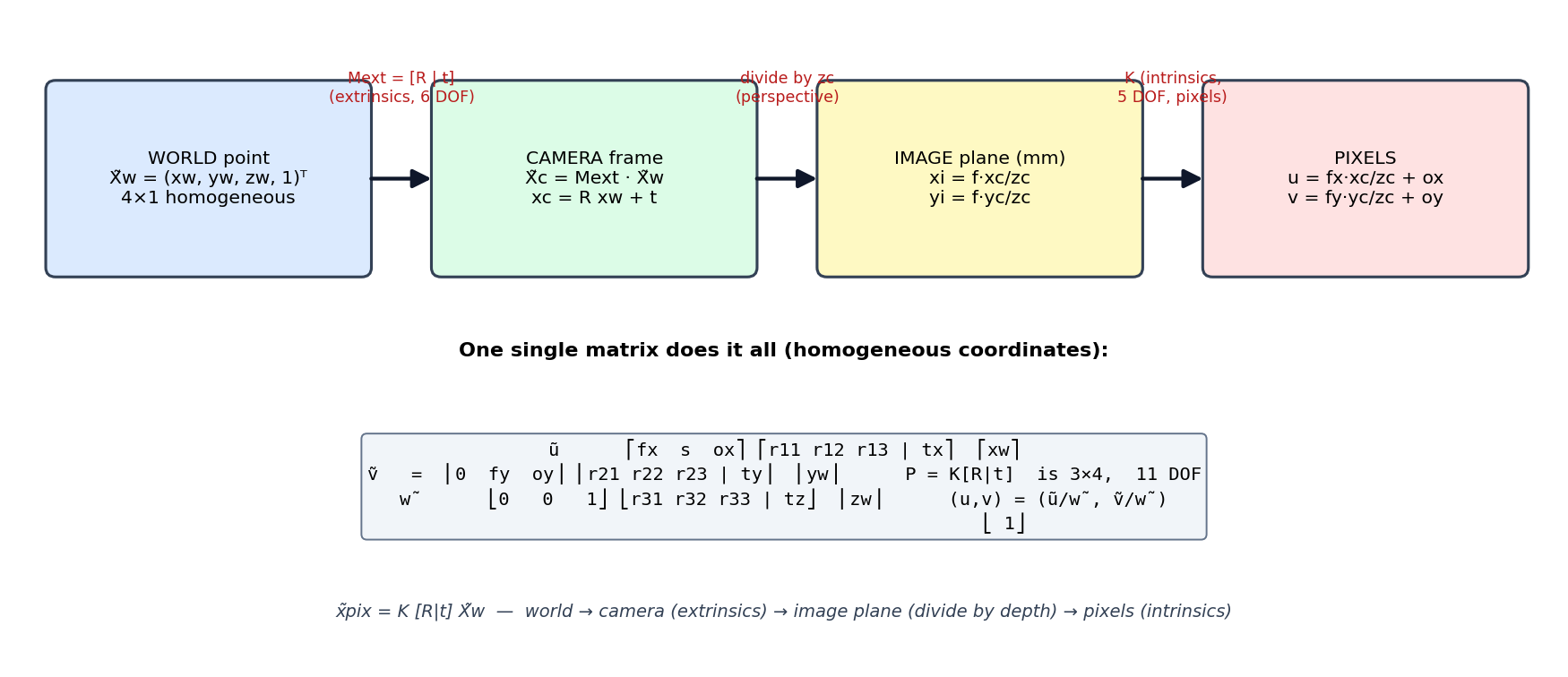
The four-stage projection pipeline — world point, extrinsic transform [R|t], perspective division, intrinsic matrix K — and the single combined matrix P = K[R|t] with the final homogeneous division. বাংলা: চার-ধাপের projection pipeline — world point, extrinsic [R|t], perspective ভাগ, intrinsic K — আর সব মিলিয়ে একটাই matrix P = K[R|t], শেষে homogeneous ভাগ।
This is the chapter on one page. Each box is a coordinate frame, each arrow a matrix (or the one division). If an exam question confuses you, place it on this diagram first: "extrinsics" live on the first arrow, "intrinsics" on the last, and the perspective division sits in the middle — which is why the extrinsic matrix alone can never reach pixel coordinates (trial-exam T/F).
বাংলা: পুরো chapter এক পাতায়। প্রতিটা বাক্স একটা coordinate frame, প্রতিটা তীর একটা matrix (বা সেই একটা ভাগ)। প্রশ্নে গুলিয়ে গেলে আগে এই ছবিতে বসান: extrinsic প্রথম তীরে, intrinsic শেষ তীরে — মাঝের ভাগটা পেরোনো ছাড়া extrinsic একা কখনো pixel-এ পৌঁছায় না (trial-exam-এর T/F-এর উত্তর)।
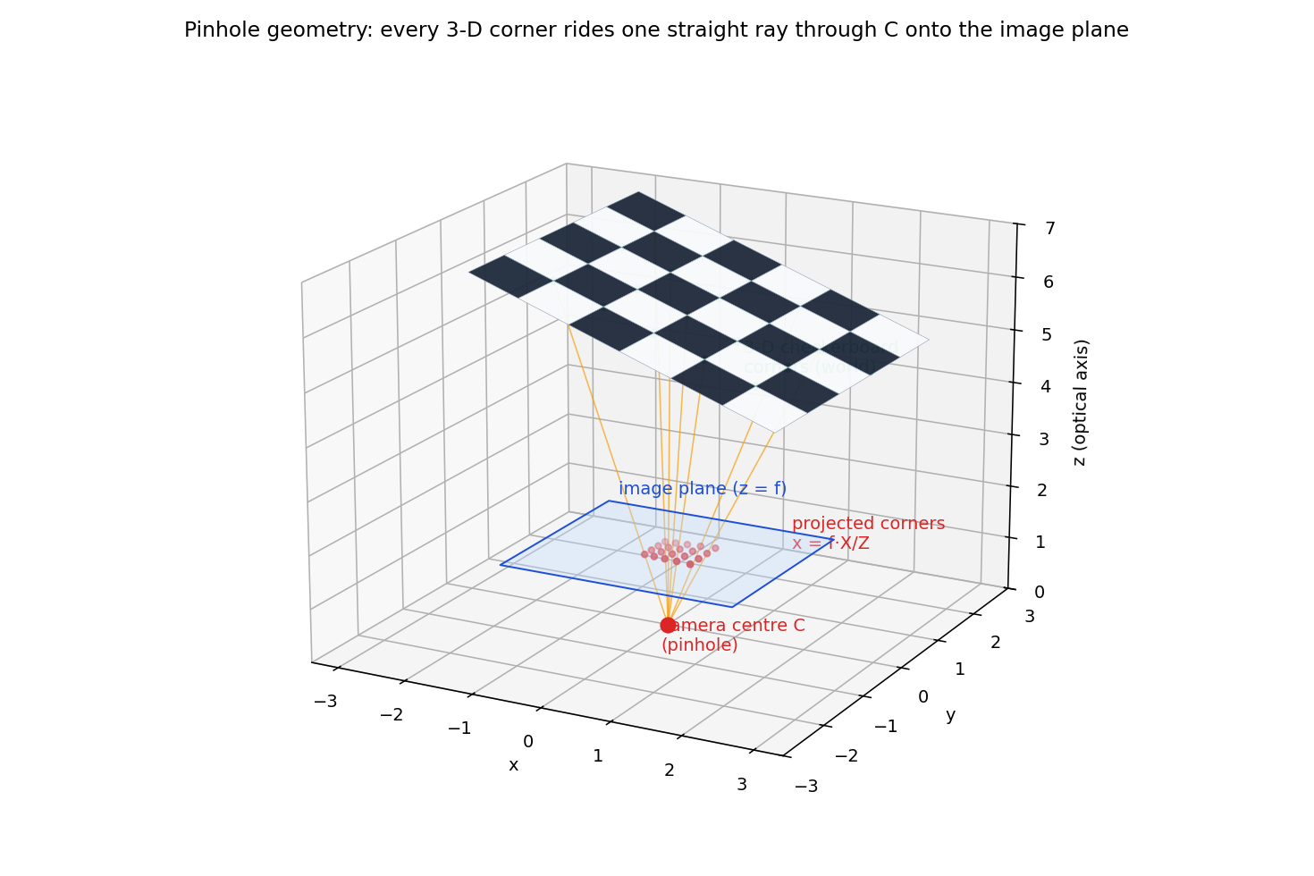
A 3-D view of the pinhole model: world checkerboard corners (green), straight rays through the camera center C (orange), and their intersections with the image plane at z = f (red) — central projection x = f·X/Z in action. বাংলা: Pinhole model-এর 3-D দৃশ্য: world-এর checkerboard কোণা (সবুজ), ক্যামেরা-কেন্দ্র C-এর ভেতর দিয়ে সরল রশ্মি (কমলা), আর z = f সমতলে তাদের ছেদবিন্দু (লাল) — central projection x = f·X/Z চোখের সামনে।
Every red point is "its green point, divided by depth, scaled by f". Note how the tilted board projects to a perspectively foreshortened pattern — the far columns are squeezed together. Calibration is the inverse riddle: given only the red points (in pixels) and the board geometry, recover where C is and what f, principal point etc. are.
বাংলা: প্রতিটা লাল বিন্দু = "তার সবুজ বিন্দু ÷ depth × f"। কাত করা board-টা ছবিতে perspective-এ চাপা পড়েছে — দূরের কলামগুলো ঘেঁষাঘেঁষি। Calibration হলো এর উল্টো ধাঁধা: শুধু লাল বিন্দু (pixel-এ) আর board-এর জ্যামিতি দেখে C, f, principal point বের করা।
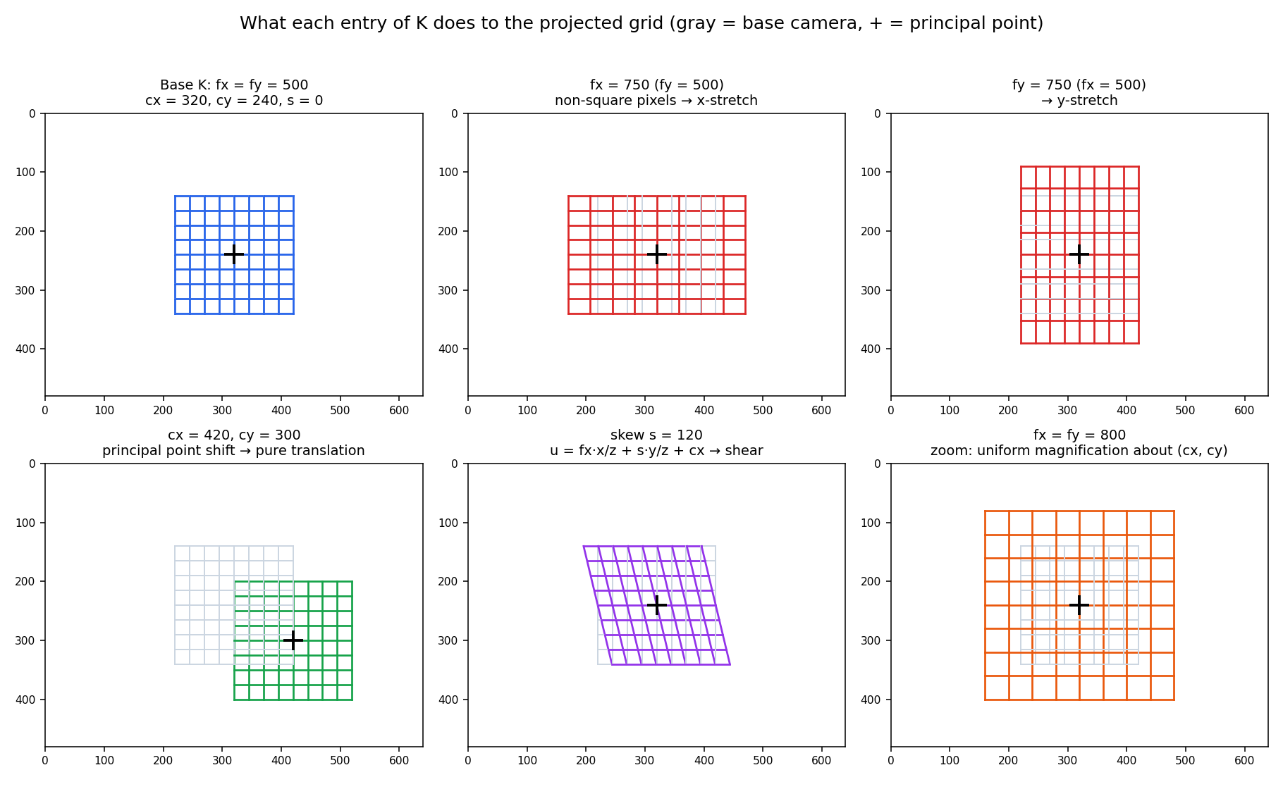
Six panels: the base camera (gray reference grid in each panel) versus a camera with one K entry changed — fx stretch, fy stretch, principal-point shift, skew shear, and uniform zoom. বাংলা: ছয়টা প্যানেল: ভিত্তি ক্যামেরা (ধূসর reference grid) বনাম K-এর একটা করে ঘর বদলানো ক্যামেরা — fx টান, fy টান, principal point সরানো, skew-এর shear, আর সমান zoom।
This is the operational meaning of K's five numbers. fx alone = horizontal stretch (non-square pixels); cx, cy = pure image translation; s = shear (u acquires a y-dependence); fx = fy increased together = zoom about the principal point. If you can sketch these five effects, you understand K.
বাংলা: K-এর পাঁচটা সংখ্যার হাতে-কলমে মানে: fx একা = পাশে টান (আয়তাকার pixel), cx/cy = পুরো ছবি সরে যাওয়া, s = shear (u-এর মধ্যে y ঢুকে পড়ে), fx আর fy একসাথে বাড়ালে = principal point ঘিরে zoom। এই পাঁচ প্রভাব আঁকতে পারা মানেই K বোঝা।
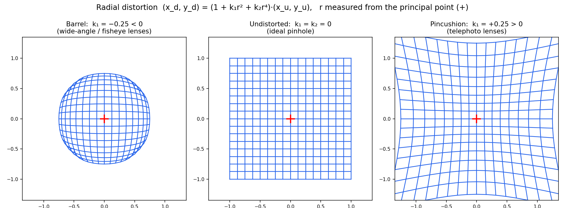
The model (x_d, y_d) = (1 + k₁r² + k₂r⁴)·(x_u, y_u) applied to a perfect grid: barrel (k₁ = −0.25), undistorted, pincushion (k₁ = +0.25). The red cross is the principal point — the origin of r. বাংলা: একটা নিখুঁত grid-এ সূত্র (1 + k₁r² + k₂r⁴) প্রয়োগ: barrel (k₁ = −0.25), distortion-হীন, pincushion (k₁ = +0.25)। লাল ক্রস principal point — r সেখান থেকেই মাপা।
Center lines stay almost straight, edge lines bend hard — because the correction factor grows with r². Barrel = wide-angle (outward bow, factor < 1 pulls points inward... so image content appears bulged), pincushion = telephoto. Exam phrasing to remember: "the coordinate origin of the distortion model is the principal point, because it is the center of the radial distortion."
বাংলা: মাঝের রেখা প্রায় সোজা, কিনারার রেখা বেশি বাঁকা — কারণ প্রভাবটা r²-এর সাথে বাড়ে। Barrel = wide-angle, pincushion = telephoto। পরীক্ষার বাক্য: "distortion model-এর origin হলো principal point, কারণ সেটাই radial distortion-এর কেন্দ্র।"
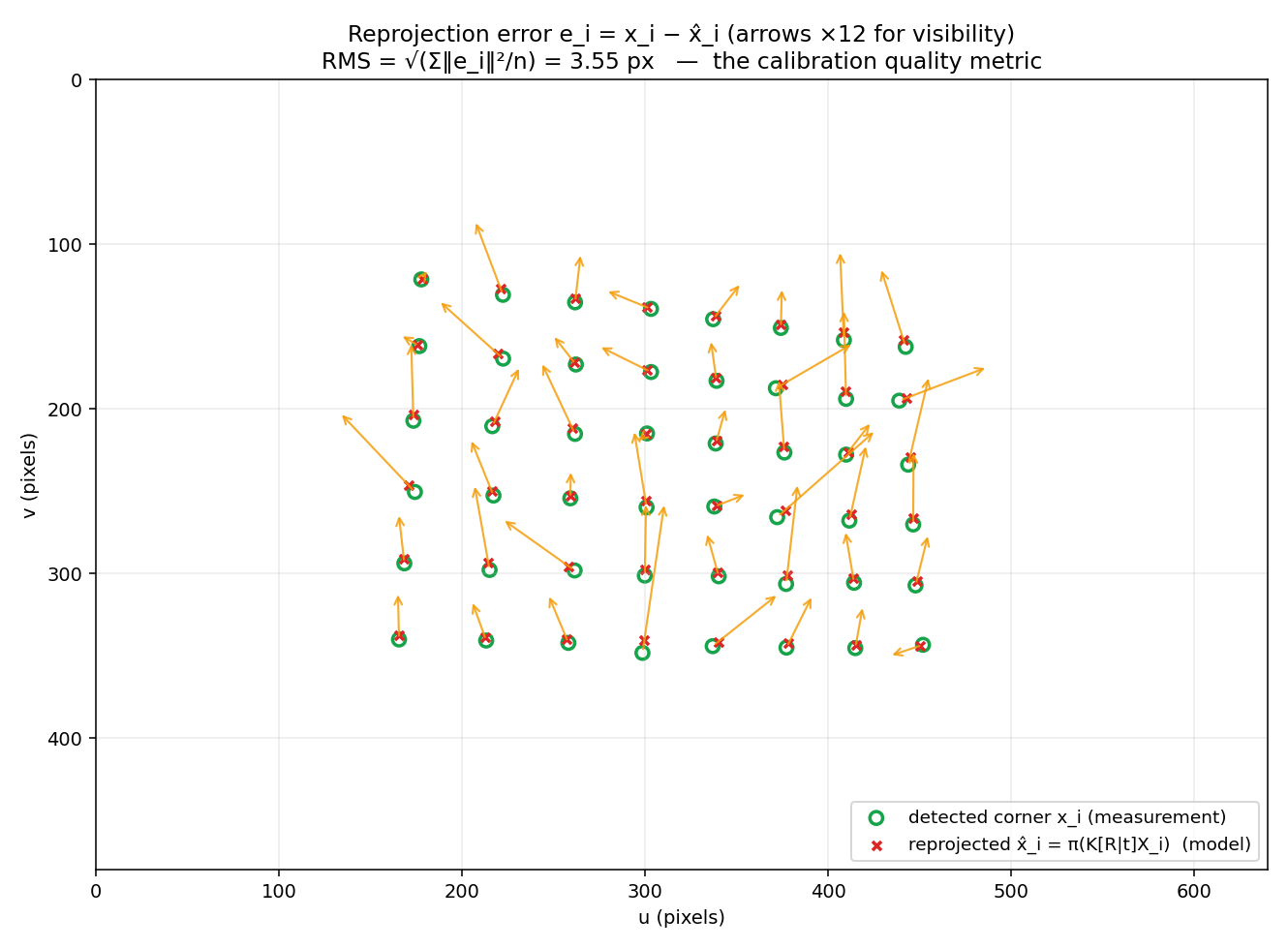
Detected checkerboard corners (green circles) versus corners reprojected through a slightly mis-calibrated camera (red crosses); orange arrows are the error vectors (magnified), with the resulting RMS in the title. বাংলা: শনাক্ত করা কোণা (সবুজ বৃত্ত) বনাম সামান্য ভুল-calibrated ক্যামেরা দিয়ে reprojected কোণা (লাল ক্রস); কমলা তীরগুলো error vector (বড় করে আঁকা), শিরোনামে RMS।
Read calibration health from the error pattern, not just the RMS: a systematic swirl or radial trend (as here — fx is 6 px too large, cy 3 px off) means a model/parameter bias; random isotropic arrows mean you've hit the detection-noise floor. This figure is the cost function of Zhang refinement and bundle adjustment, drawn.
বাংলা: শুধু RMS নয়, error-এর নকশা পড়ুন: তীরগুলো নিয়মমাফিক ঘুরলে/ছড়ালে (এখানে fx ৬ px বেশি, cy ৩ px সরানো) বুঝবেন model বা parameter-এ পক্ষপাত আছে; আর এলোমেলো সমান তীর মানে আপনি detection noise-এর মেঝেতে পৌঁছে গেছেন। এই ছবিটাই Zhang refinement আর bundle adjustment-এর cost function — আঁকা অবস্থায়।
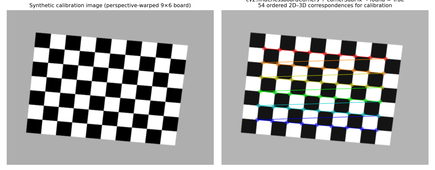
Left: a synthetic, perspective-warped 9×6 checkerboard image. Right: cv2.findChessboardCorners + cornerSubPix finds all 54 inner corners in a guaranteed order — instant 2D–3D correspondences for calibration. বাংলা: বাঁয়ে: কৃত্রিম, perspective-এ বাঁকানো 9×6 checkerboard। ডানে: cv2.findChessboardCorners + cornerSubPix ৫৪টা ভেতরের কোণাই নির্দিষ্ট ক্রমে খুঁজে পেয়েছে — calibration-এর জন্য তৈরি 2D–3D জোড়া।
Why checkerboards? Corners are localizable to sub-pixel accuracy (saddle points of intensity), the grid's known ordering solves the matching problem for free, and the printed square size injects the metric scale. The rainbow line shows the detection order — that order is what lets us assign each corner its board coordinate (i·25mm, j·25mm, 0).
বাংলা: Checkerboard কেন? কোণাগুলো sub-pixel নিখুঁততায় বের করা যায় (intensity-র saddle point), grid-এর জানা ক্রম matching সমস্যাটা ফ্রি-তে সমাধান করে দেয়, আর ছাপানো ঘরের মাপ metric scale ঢুকিয়ে দেয়। রামধনু রেখাটা detection-ক্রম — সেই ক্রমেই প্রতিটা কোণাকে তার board-স্থানাঙ্ক (i·25mm, j·25mm, 0) দেওয়া হয়।
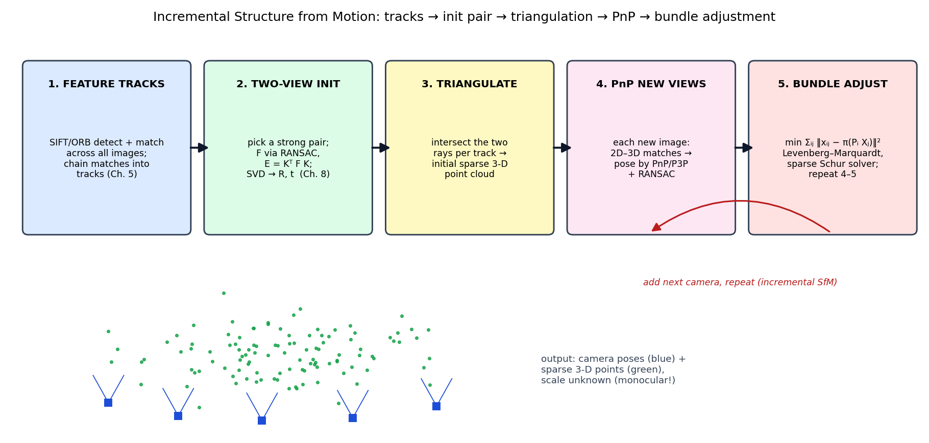
Incremental Structure from Motion: feature tracks → two-view initialization (F → E → R, t) → triangulation → PnP registration of each new camera → bundle adjustment, looping until all images are placed. Below: the output — camera poses + a sparse point cloud, scale unknown. বাংলা: Incremental SfM: feature track → দুই-view শুরু (F → E → R, t) → triangulation → প্রতিটা নতুন ক্যামেরার জন্য PnP → bundle adjustment, সব ছবি বসা পর্যন্ত চক্র। নিচে ফলাফল: ক্যামেরার অবস্থান + sparse point cloud — scale অজানা।
Each stage reuses an earlier chapter: tracks = Chapter 5 (SIFT), init pair = Chapter 8 (F/RANSAC), triangulation/PnP/BA = this chapter. Keep the loop in mind: PnP and BA alternate as cameras are added — BA is run repeatedly, not once at the end.
বাংলা: প্রতিটা ধাপ আগের কোনো chapter-এর পুনর্ব্যবহার: track = Chapter 5 (SIFT), শুরুর জোড়া = Chapter 8 (F/RANSAC), triangulation/PnP/BA = এই chapter। চক্রটা মনে রাখুন: ক্যামেরা যোগ হতে হতে PnP আর BA পালা করে চলে — BA শুধু শেষে একবার নয়, বারবার।
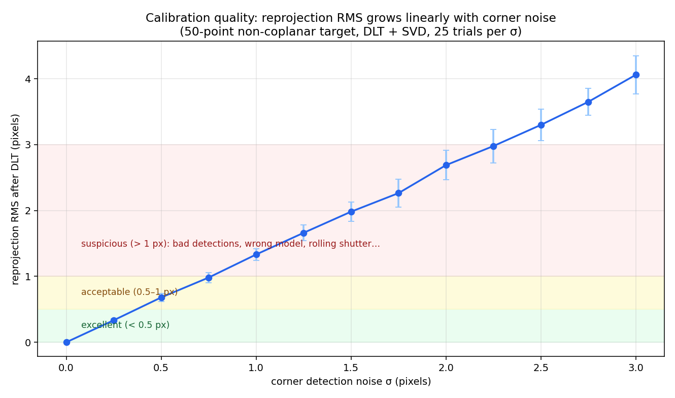
A synthetic DLT experiment: corners of a 50-point non-coplanar target are perturbed with Gaussian noise of growing σ; the reprojection RMS after DLT grows linearly with σ. Colored bands mark the practical quality zones. বাংলা: কৃত্রিম DLT পরীক্ষা: ৫০-বিন্দুর অ-সমতলীয় target-এর কোণায় ক্রমবর্ধমান σ-এর Gaussian noise; DLT-র পরে reprojection RMS σ-এর সাথে সরলরৈখিকভাবে বাড়ে। রঙিন ব্যান্ডগুলো মানের ব্যবহারিক অঞ্চল।
Two lessons. First, RMS inherits the detector's noise level linearly — sub-pixel corner detection is what buys sub-pixel calibration. Second, note the RMS slightly exceeds σ here: plain DLT minimizes an algebraic error, not the geometric reprojection error, so its solution is not the geometric optimum — exactly why every real pipeline follows the linear estimate with non-linear refinement (and why Hartley normalization matters).
বাংলা: দুটো শিক্ষা: (১) RMS detector-এর noise-কে সরলরৈখিকভাবে উত্তরাধিকার পায় — sub-pixel corner detection-ই sub-pixel calibration কেনে। (২) লক্ষ করুন RMS এখানে σ-এর চেয়ে একটু বেশি: সরল DLT algebraic error কমায়, geometric reprojection error নয় — সেজন্যই বাস্তব pipeline-এ linear অনুমানের পরে non-linear refinement বাধ্যতামূলক।
§6 Algorithms & Code¶
6.1 Forward projection — the worked example as code¶
import numpy as np

def project(K, R, t, X_w):
    """World point -> pixel, with explicit homogeneous division."""
    X_c = R @ X_w + t                  # stage 1: world -> camera
    assert X_c[2] > 0, "point behind the camera!"
    uvw = K @ X_c                      # stage 2+3: homogeneous pixel
    return uvw[:2] / uvw[2]            # stage 4: NEVER forget this division

K = np.array([[400, 0, 320], [0, 400, 240], [0, 0, 1]], float)
R = np.array([[0, 0, 1], [0, 1, 0], [-1, 0, 0]], float)   # Ry(90 deg)
t = np.array([0, 0, 6], float)
print(project(K, R, t, np.array([4, 1, 1.0])))            # [520. 440.]
print(-R.T @ t)                                           # camera centre [6. 0. 0.]
Step-by-step. Three lines mirror §4.7 exactly: rigid motion, K multiplication, homogeneous division. The assertion catches the classic failure (\(zc \le 0\)).
বাংলা: §4.7-এর তিন ধাপ তিন লাইনে। assert-টা ধরে ফেলে ক্লাসিক বিপদ: \(zc \le 0\) মানে বিন্দু ক্যামেরার পেছনে বা ঠিক pinhole-সমতলে — projection অর্থহীন। শেষ লাইনের ভাগটা বাদ দিলে উত্তর হবে homogeneous সংখ্যা, pixel নয়।
6.2 DLT from scratch (the §4.8 derivation, runnable)¶
def calibrate_dlt(X_w, uv):
    """X_w: (n,3) known 3-D points (NOT coplanar), uv: (n,2) pixels, n >= 6.
    Returns the 3x4 projection matrix P (up to scale)."""
    n = len(X_w)
    A = np.zeros((2 * n, 12))
    for i in range(n):
        X = np.append(X_w[i], 1.0)            # homogeneous (4,)
        u, v = uv[i]
        A[2*i,     0:4] = X                   #  X~ . p1  - u (X~ . p3) = 0
        A[2*i,     8:12] = -u * X
        A[2*i + 1, 4:8] = X                   #  X~ . p2  - v (X~ . p3) = 0
        A[2*i + 1, 8:12] = -v * X
    _, _, Vt = np.linalg.svd(A)
    return Vt[-1].reshape(3, 4)               # smallest right singular vector
Step-by-step. Each correspondence writes the two §4.8 equations into two rows of A; the SVD's last right singular vector minimizes \(\|Ap\|\) under \(\|p\| = 1\). Production tip: normalize coordinates first (Hartley) and refine with scipy.optimize.least_squares on the true reprojection error.
বাংলা: প্রতি জোড়া থেকে §4.8-এর দুটো সমীকরণ A-এর দুটো সারিতে; SVD-র শেষ ডান singular vector-ই \(\|p\|=1\) শর্তে \(\|Ap\|\) minimize করে। মনে রাখুন: বিন্দুগুলো অ-সমতলীয় হতে হবে, আর ভালো ফলের জন্য আগে Hartley normalization, পরে আসল reprojection error-এ refinement।
6.3 Decomposing P into K, R, t (RQ)¶
from scipy.linalg import rq

def decompose_P(P):
    M = P[:, :3]                       # left 3x3 block = K R
    K, R = rq(M)                       # upper-triangular x orthonormal
    S = np.diag(np.sign(np.diag(K)))   # fix signs: K diagonal must be > 0
    K, R = K @ S, S @ R                # (S @ S = I, so K R is unchanged)
    if np.linalg.det(R) < 0:           # keep det(R) = +1
        K, R = -K, -R
    t = np.linalg.inv(K) @ P[:, 3]     # last column: p4 = K t
    return K / K[2, 2], R, t           # normalize overall scale
Step-by-step. RQ on the left block, a sign-fixing diagonal S (RQ is unique only up to signs), determinant check for a proper rotation, then \(t = K^{-1}p_{4}\) and scale normalization \(K[2,2] = 1\). This is trial-exam Q9a as five lines of code.
বাংলা: বাঁ 3×3 block-এ RQ → চিহ্ন ঠিক করা (K-এর কর্ণ ধনাত্মক, S²=I বলে গুণফল অটুট) → \(\det R = +1\) নিশ্চিত করা → \(t = K^{-1}p_{4}\) → \(K[2,2] = 1\)। Q9a-র উত্তরটাই পাঁচ লাইনের কোড।
6.4 Zhang's method with OpenCV (the practical workhorse)¶
import cv2, glob
import numpy as np

pattern = (9, 6)                                  # inner corners
objp = np.zeros((np.prod(pattern), 3), np.float32)
objp[:, :2] = np.indices(pattern).T.reshape(-1, 2) * 25.0   # 25 mm squares -> metric scale!

obj_pts, img_pts = [], []
for fname in glob.glob("calib/*.png"):            # >= 3 views, better 10-20
    gray = cv2.imread(fname, cv2.IMREAD_GRAYSCALE)
    ok, corners = cv2.findChessboardCorners(gray, pattern)
    if not ok:
        continue
    corners = cv2.cornerSubPix(gray, corners, (5, 5), (-1, -1),
                               (cv2.TERM_CRITERIA_EPS + cv2.TERM_CRITERIA_MAX_ITER, 30, 1e-3))
    obj_pts.append(objp); img_pts.append(corners)

rms, K, dist, rvecs, tvecs = cv2.calibrateCamera(obj_pts, img_pts,
                                                 gray.shape[::-1], None, None)
print("RMS reprojection error [px]:", rms)        # want < 0.5
print("K =\n", K)
print("dist (k1 k2 p1 p2 k3) =", dist.ravel())
undist = cv2.undistort(cv2.imread("test.png"), K, dist)
Step-by-step. objp holds the board coordinates with \(zw = 0\) (planar target — Zhang!) in millimeters; one (rvec, tvec) pair comes back per view (extrinsics change per photo, intrinsics are shared). rms is exactly §4.11's metric. The printed square size (25 mm) is what makes tvecs metric — the scale-ambiguity escape hatch.
বাংলা: objp-তে board-স্থানাঙ্ক, \(zw = 0\) (সমতল target — তাই এটা Zhang)। প্রতি ছবির জন্য আলাদা (rvec, tvec) ফেরত আসে কিন্তু K, dist একটাই — intrinsic সব view-তে ভাগ করা, extrinsic প্রতি view-তে নতুন (Q9b-র জীবন্ত প্রমাণ)। rms হলো §4.11-এর মাপকাঠি — 0.5-এর নিচে চাই। আর ২৫ মিমি ঘরের মাপটাই tvecs-কে আসল মিলিমিটারে আনে — scale ambiguity থেকে মুক্তির পথ।
6.5 Linear triangulation¶
def triangulate(P1, P2, x1, x2):
    """P1,P2: 3x4 camera matrices; x1,x2: (u,v) pixels of one correspondence."""
    A = np.array([x1[0] * P1[2] - P1[0],
                  x1[1] * P1[2] - P1[1],
                  x2[0] * P2[2] - P2[0],
                  x2[1] * P2[2] - P2[1]])
    _, _, Vt = np.linalg.svd(A)
    X = Vt[-1]
    return X[:3] / X[3]                # homogenize the 3-D point
Step-by-step. Each view contributes rows \(u\cdot p_{3}^{T} - p_{1}^{T}\) and \(v\cdot p_{3}^{T} - p_{2}^{T}\) (the DLT pattern again); the SVD null vector is the homogeneous 3-D point; the final division homogenizes. The pseudo-inverse formulation \(x = (A^{T}A)^{-1}A^{T}b\) from the lecture is the inhomogeneous twin.
বাংলা: প্রতিটা view দেয় \(u\cdot p_{3}^{T} - p_{1}^{T}\) ধাঁচের দুটো সারি — আবারও DLT নকশা; SVD-র null vector-ই homogeneous 3-D বিন্দু; শেষে ভাগ। Lecture-এর pseudo-inverse রূপ \(x = (A^{T}A)^{-1}A^{T}b\) একই জিনিসের অ-homogeneous যমজ।
6.6 Mini SfM pipeline (pseudo-code with real anchors)¶
# 1. Features & tracks:      SIFT/ORB detect+match all pairs  -> tracks    (Ch. 5)
# 2. Init pair:               F, _ = cv2.findFundamentalMat(x1, x2, cv2.FM_RANSAC)
#                            E = K.T @ F @ K                                (Ch. 8)
#                            _, R, t, _ = cv2.recoverPose(E, x1, x2, K)   # chirality test inside
# 3. Triangulate tracks:     cv2.triangulatePoints(P1, P2, x1.T, x2.T)
# 4. Register next camera:   _, rvec, tvec, inl = cv2.solvePnPRansac(X3d, x2d, K, dist)
# 5. Bundle adjustment:      scipy.optimize.least_squares(residual, params,
#                                jac_sparsity=S, method="trf")   # S encodes the BA sparsity
# 6. goto 4 until all images placed;  export point cloud (.ply) for MeshLab
Notes. recoverPose resolves the four-fold (R, t) ambiguity of E by checking which combination puts points in front of both cameras. jac_sparsity is the small-scale stand-in for the Schur-complement structure of §4.15. The cloud's scale is arbitrary unless step 2's t is given a metric length from outside.
বাংলা: recoverPose E-এর চারটা সম্ভাব্য (R, t) জোড়ার মধ্যে সেটাই বেছে নেয় যেটায় বিন্দুরা দুই ক্যামেরারই সামনে পড়ে। jac_sparsity হলো §4.15-এর Schur-গঠনের ছোট সংস্করণ। আর মনে রাখুন: বাইরে থেকে মাপ না দিলে পুরো cloud-এর scale ইচ্ছামূলক।
§7 Trial-Exam Mapping¶
| Trial-exam item | What you must know | Where in this chapter |
|---|---|---|
| Q9a How are intrinsic parameters extracted from a projection matrix? | Left 3×3 block of P is K·R → RQ/QR factorization → upper-triangular K + orthonormal R; then t = K⁻¹·p₄ | §4.9, code §6.3 |
| Q9b Two types of camera parameters, two examples each, how often do they change? | Extrinsic: R, t (position/orientation) — change with every movement/frame. Intrinsic: focal length, principal point, pixel size, skew — change only with lens/sensor (zoom) | §2.2, §4.5–4.6 |
| Q9c T/F: "extrinsic matrix maps world coordinates directly to pixels" | False — [R|t] reaches only the camera frame; pixels need K too (P = K[R|t]) | §4.1–4.2, pipeline figure |
| Q9c T/F: "radial distortion is corrected by an affine transformation" | False — the model contains r², r⁴: the scaling varies with radius, which no affine (globally linear) map can express | §4.10, distortion figure |
| Q9c T/F: "depth can be computed from disparity using triangulation" | True — z = b·f/d is exactly similar-triangle triangulation (Ch. 8) | §4.14 |
Model answer (Q9b, two sentences): "Cameras have extrinsic parameters — position and orientation (R, t) — which change every time the camera moves, i.e. potentially every frame; and intrinsic parameters — focal length, principal point, pixel size/aspect, skew — which describe the camera's internal geometry and only change when the optics change, e.g. when zooming or swapping the lens."
বাংলা: Q9 পুরোটাই এই chapter থেকে: (a) RQ দিয়ে P ভাঙা — §4.9-এর তিন-লাইনের উত্তর মুখস্থ; (b) দুই ধরনের parameter আর কখন বদলায় — extrinsic প্রতি নড়াচড়ায়, intrinsic প্রতি lens-বদলে; © তিনটা T/F-এর ফাঁদ — extrinsic একা pixel-এ পৌঁছায় না (F), distortion affine নয় (F), disparity থেকে depth = triangulation (T)।
§8 Mock Exam — 20 Questions¶
Answer everything on paper first; full worked solutions follow in §8.5. Tier A = basics, B = intuition, C = harder computation/derivation, D = transfer questions slightly beyond the lecture (typical for a tough oral or a "Transfer" section in the written exam).
Tier A — Basic (definitions & direct formula use)¶
A1. Cameras have two types of parameters. Name both types, give two examples of each, and state how often each type changes. (This is trial-exam Q9b — answer in at most four sentences.)
A2. Write out the calibration matrix K with all five entries. For each entry give its meaning and its unit. State the relation between the metric focal length f (in mm) and fx (in pixels), and say exactly when \(fx \neq fy\).
A3. The projection matrix \(P = K[R|t]\). (a) What size is P? (b) Count its degrees of freedom two ways: from the camera parameters, and from the matrix entries. © Why is P only defined up to scale?
A4. Project the world point \(xw = (2, 1, 5)^{T}\) with
Show the homogeneous pixel and the final division.
A5. Given
(a) Verify that R is a valid rotation matrix (state and check all required properties). (b) Write down \(R^{-1}\) without doing any matrix inversion, and justify. © How many degrees of freedom does a rotation matrix have, and why?
Tier B — Intuitive (why / when)¶
B6. The projection equations contain a division by depth, yet the whole chapter insists projection is "one linear matrix multiplication". Explain how homogeneous coordinates resolve this contradiction, say where the depth hides inside \(K\cdot [R|t]\cdot \tilde{x}w\), and name the single most common exam mistake connected to this.
B7. Why is K upper triangular — and why is that exactly the property that makes the RQ decomposition of \(M = KR\) work? Why does the implementation additionally have to fix the signs of K's diagonal?
B8. Why does DLT calibration fail when all 3-D calibration points lie in one plane? And how does Zhang's method nevertheless calibrate from a planar checkerboard?
B9. Why is the reprojection error the universal quality metric of this chapter (give at least three reasons)? Interpret: calibration run 1 reports RMS = 0.3 px, run 2 reports RMS = 2.0 px. And what is the diagnostic difference between error arrows forming a systematic radial pattern versus random isotropic arrows?
B10. A monocular SfM reconstruction of a building comes out geometrically perfect but in meaningless units. Explain why no algorithm could have done better, give the formal one-line argument, and name three different ways to inject true metric scale. Why is the printed square size of a checkerboard already sufficient?
Tier C — Harder (multi-step computation / derivation)¶
C11. DLT bookkeeping. (a) For n 2D–3D correspondences, what is the size of the DLT matrix A and how many equations does it hold? (b) Why are there only 11 effective unknowns although P has 12 entries? © Derive the minimal n. (d) For \(n = 10\): give A's size and describe exactly how p is extracted from A. (e) A student uses \(n = 100\) very accurate points — but all on the flat facade of a building. What happens, and why?
C12. Project the world point \(xw = (0.1, 0.2, 1.5)^{T}\) through the camera
(R = rotation by 90° about z.) (a) Compute xc and verify the point is in front of the camera. (b) Compute the pixel (u, v) with the homogeneous division written out. © Compute the camera center cw in world coordinates.
C13. A camera has square pixels, principal point \((ox, oy) = (320, 240)\), \(R = I\), \(t = 0\). The point \(xc = (0.5, 0.25, 2)^{T}\) is observed at pixel (520, 340). (a) Recover fx and fy from this single observation and check they are consistent with square pixels. (b) The sensor's pixel size is 5 µm. Compute the metric focal length f in mm via \(fx = mx\cdot f\). © Check the units of that formula explicitly.
C14. A lens has radial distortion \(k_{1} = -0.3\) (k₂ = p₁ = p₂ = 0). The undistorted normalized image point is \((x, y) = (0.4, 0.2)\); intrinsics: \(fx = fy = 500\), \((ox, oy) = (320, 240)\). (a) Compute the distorted normalized coordinates. (b) Compute the distorted pixel. © Compute the pixel the ideal pinhole would have produced, and the displacement caused by the lens. (d) Barrel or pincushion — justify from the numbers.
C15. Build a projection matrix from parts:
(a) Write out the full 3×4 matrix \(P = K[R|t]\) with all 12 numbers. (b) Project the world origin with it. © Give the camera center cw. (d) Multiply P by \(k = 2\) and re-project the origin — what do you observe, and which fact from §4.6 does this confirm?
Tier D — Transfer (adjacent to, but beyond, the lecture)¶
D16. Compare classic DLT calibration (3-D target) and Zhang's method (planar target) as engineering trade-offs: target manufacturing, number of images, what each can/cannot estimate, error being minimized, degeneracies. Then derive the count showing why Zhang needs at least 3 views of the plane, and state the extra condition on those views.
D17. A student calibrates a camera by waving a checkerboard quickly in front of a rolling-shutter CMOS camera. The RMS is mysteriously high and fx comes out differently in different runs. Explain what rolling shutter does to the single-pose-per-image assumption, why it biases calibration (and SfM), and give at least three practical remedies.
D18. A 190° fisheye lens is calibrated with the Brown–Conrady model — the optimization diverges. Explain why the polynomial model fundamentally cannot represent such a lens (consider \(r = f\cdot \tan \theta\) as θ → 90°), write down the equidistant fisheye model and show it stays finite at θ = 90°, and name the practical consequence for OpenCV users.
D19. PnP inside RANSAC. (a) What is the minimal number of 2D–3D correspondences for camera pose with known K, and what is this solver called? (b) How many solutions can the minimal problem have and how is the ambiguity resolved? © Using \(N = \log (1 - p)/\log (1 - w^{s})\) with inlier ratio \(w = 0.5\) and success probability \(p = 0.99\), compute the required RANSAC iterations for a minimal \(s = 3\) solver versus a 6-point DLT-style solver, and draw the engineering conclusion.
D20. Bundle adjustment with \(M = 100\) cameras (shared, fixed intrinsics) and \(N = 50,000\) points. (a) Count the unknowns. (b) Explain why each residual's Jacobian row touches only 9 of them, and what the resulting Jacobian/normal-equation structure looks like. © Explain in two or three sentences how the Schur complement exploits this. (d) What is the gauge freedom of the problem and how is it usually fixed?
§8.5 Solutions¶
Tier A¶
A1.
Extrinsic / external parameters describe the camera's pose in the world — examples: the rotation matrix R (orientation) and the translation vector t (position; equivalently the camera center \(cw = -R^{T}t\)). They change every time the camera moves — for video, potentially every frame.
Intrinsic / internal parameters describe the camera's internal geometry — examples: focal length fx, fy (or f), principal point (ox, oy) (also pixel densities, skew, distortion coefficients k₁, k₂). They stay constant while the lens and sensor stay the same and only change when the optics change (zooming, swapping the lens).
বাংলা: Extrinsic = ক্যামেরার ভঙ্গি (R, t) — নড়লেই বদলায়; intrinsic = ক্যামেরার গঠন (focal length, principal point) — lens বদলালে তবেই বদলায়। দুটো উদাহরণ আর "কখন বদলায়" — এই তিনটা জিনিস বললেই পুরো নম্বর।
A2.
| Entry | Meaning | Unit |
|---|---|---|
| \(fx = mx\cdot f\) | focal length in x, in pixel units | pixels |
| \(fy = my\cdot f\) | focal length in y, in pixel units | pixels |
ox |
principal point, x (optical axis ∩ sensor) | pixels |
oy |
principal point, y | pixels |
s |
skew — non-perpendicularity of pixel axes | pixels (≈ 0 in modern cameras) |
Relation: \(fx = mx\cdot f\), where f is in mm and mx is the pixel density in pixels per mm — so \((px/mm)\cdot mm = px\), the mm cancels. \(fx \neq fy\) exactly when the pixels are not square (\(mx \neq my\), rectangular photosites).
বাংলা: K-এর পাঁচটা সংখ্যাই pixel এককে; \(fx = mx\cdot f\)-এ মিমি কেটে গিয়ে pixel থাকে। \(fx \neq fy\) মানেই pixel আয়তাকার — এটা lens-এর দোষ নয়, sensor-এর গড়ন।
A3.
(a) P is 3×4.
(b) From parameters: 5 intrinsic (fx, fy, ox, oy, s) + 6 extrinsic (3 rotation + 3 translation) = 11. From entries: 3·4 = 12 entries − 1 for the irrelevant overall scale = 11. The two counts agree — P encodes exactly the camera parameters.
© P acts on homogeneous vectors: \((kP)\cdot \tilde{x}w = k\cdot (P\cdot \tilde{x}w)\), and the homogeneous division cancels the factor k, so P and kP produce identical pixels.
বাংলা: ৫ + ৬ = ১১ = ১২ − ১ — দুই পথের হিসাব মিলে যাওয়াটাই উত্তরের প্রাণ। Scale-টা ছবিতে অদৃশ্য, কারণ ভাগের সময় k কেটে যায়।
A4. With \(R = I, t = 0\) we have \(xc = xw = (2, 1, 5)^{T}\), depth \(zc = 5 > 0\) ✓.
       ⎡400   0  320⎤ ⎡2⎤   ⎡400·2 + 320·5⎤   ⎡ 800 + 1600⎤   ⎡2400⎤
ũ   =  ⎢  0 400  240⎥ ⎢1⎥ = ⎢400·1 + 240·5⎥ = ⎢ 400 + 1200⎥ = ⎢1600⎥
       ⎣  0   0    1⎦ ⎣5⎦   ⎣            5⎦   ⎣          5⎦   ⎣   5⎦

(u, v) = (2400/5, 1600/5) = (480, 320)
বাংলা: Homogeneous pixel (2400, 1600, 5), তারপর ৫ দিয়ে ভাগ → (480, 320)। ভাগটা বাদ দিলে শূন্য নম্বর — এই chapter-এর এক নম্বর ফাঁদ।
A5. (a) Required properties: orthonormal (\(R^{T}R = I\): each column unit length, columns mutually orthogonal) and det R = +1. Columns: \(c_{1} = (0,1,0)^{T}, c_{2} = (-1,0,0)^{T}, c_{3} = (0,0,1)^{T}\) — each has length 1; \(c_{1}\cdot c_{2} = 0, c_{1}\cdot c_{3} = 0, c_{2}\cdot c_{3} = 0\) ✓. Determinant (expansion along the first row): \(\det = 0\cdot (0\cdot 1 - 0\cdot 0) - (-1)\cdot (1\cdot 1 - 0\cdot 0) + 0 = +1\) ✓ — a proper rotation, no reflection. (b) For any orthonormal matrix \(R^{-1} = R^{T}\):
© 3 DOF: 9 entries minus 6 orthonormality constraints (3 unit-length conditions + 3 orthogonality conditions) — e.g. three rotation angles. বাংলা: যাচাইয়ের তালিকা: কলামগুলোর দৈর্ঘ্য ১, পরস্পর লম্ব, det = +1। উল্টানো বিনা খরচে: \(R^{-1} = R^{T}\)। DOF = ৯ − ৬ = ৩।
Tier B¶
B6.
The map \((u, v) = (fx\cdot xc/zc + ox, fy\cdot yc/zc + oy)\) is non-linear because of the division by zc. Homogeneous coordinates postpone that division instead of removing it: we compute a homogeneous pixel \((\tilde{u}, \tilde{v}, \tilde{w}) = K[R|t]\cdot \tilde{x}w\) — purely linear — and define the Euclidean pixel as \((\tilde{u}/\tilde{w}, \tilde{v}/\tilde{w})\). The depth hides in the third row of K, (0 0 1): it simply copies zc into w̃, so the final homogenization is the perspective division. Everything non-linear is concentrated in one final step; everything before it is matrix algebra.
The classic exam mistake: forgetting to divide by w̃ and reporting the homogeneous triple as the pixel.
বাংলা: Homogeneous কৌশল ভাগটাকে বাতিল করে না — জমিয়ে রাখে। K-এর তৃতীয় সারি (0 0 1) depth-টাকে w̃-তে কপি করে, শেষের ভাগটাই perspective। ভাগ ভুলে গেলে উত্তর pixel নয়, তিনটা অর্থহীন সংখ্যা।
B7. K is upper triangular because the image-plane→pixel map is built only from "scale by the focal lengths, shear by the skew, translate by the principal point" — it contains no rotation, so u depends on (x, y)-inputs and v only on y: zero below the diagonal. The left 3×3 block of P is \(M = KR\) — upper-triangular times orthonormal — and that is precisely the output format of the RQ decomposition, so running RQ on M must return K and R. The decomposition is only unique up to signs: for any diagonal sign matrix S with \(S^{2} = I\), \(M = (KS)(SR)\) is an equally valid factorization. We fix the ambiguity by demanding K's diagonal entries (the focal lengths) be positive — physically meaningful — and then enforce \(\det R = +1\). বাংলা: K-তে ঘূর্ণন নেই বলেই সে triangular; আর M = KR ঠিক RQ-র ছাঁচে বলেই RQ চালালে K, R আলাদা হয়। চিহ্নের স্বাধীনতা (S² = I) মেটাতে নিয়ম: focal length ধনাত্মক, det R = +1।
B8. If all points satisfy one plane equation, the image observations only constrain the homography between that plane and the image — a 3×3 object with 8 DOF — while P has 11 DOF. The DLT matrix A then has extra null space (a whole family of P's reproduces the data: you can bend the camera and compensate within the unconstrained directions), so the SVD solution is arbitrary within that family — DLT fails. Zhang turns the weakness into the method: each view of the plane gives exactly that homography \(H = K[r_{1} r_{2} t]\), and the orthonormality of \(r_{1}, r_{2}\) converts each H into 2 constraints on ω = K⁻ᵀK⁻¹, which depends on intrinsics only. Intrinsics are shared across views, so stacking ≥ 3 differently-oriented views gives ≥ 6 ≥ 5 constraints — enough to solve for ω, hence K, and then each view's R, t. বাংলা: সমতল target এক ছবিতে P-কে বাঁধতে পারে না (8 < 11 DOF) — কিন্তু K সব ছবিতে এক, তাই Zhang অনেক ছবির homography-র শর্ত জমিয়ে K বের করে। DLT-র দুর্বলতাই Zhang-এর কৌশল।
B9. Reasons: (1) it is measured in the image, in pixels — the only place where we have actual ground truth (the detected corners/features); (2) it judges all parameters jointly (K, R, t, distortion) instead of needing per-parameter ground truth nobody has; (3) it is exactly the cost function minimized by Zhang's refinement, PnP refinement and bundle adjustment, so reporting it tells you how well the optimization did; (4) it is comparable across cameras and datasets. RMS 0.3 px = excellent, sub-pixel — consistent with good corner detection; RMS 2.0 px = something is structurally wrong (mislabeled corners, wrong/missing distortion model, rolling shutter, moving board) — not just "a bit noisier". Pattern reading: a systematic radial/swirl pattern means a biased model — some parameter (fx, principal point, missing k₁) is off, and the residuals all "point" the same way; random isotropic arrows mean the model has soaked up everything explainable and you are at the detection-noise floor — the calibration is as good as the data. বাংলা: RMS ছোট মানেই শেষ নয় — তীরের নকশা দেখুন: নিয়মমাফিক ঘূর্ণি/রশ্মি-নকশা = model-এ পক্ষপাত বাকি; এলোমেলো সমান তীর = noise-এর মেঝে, আর কিছু করার নেই। 0.3 px চমৎকার; 2 px মানে কোথাও কাঠামোগত গোলমাল।
B10.
Scaling the whole world and the camera path together leaves every image unchanged: for any \(\lambda > 0\), replacing \(X_{j} \to \lambda X_{j}\) and \(t_{i} \to \lambda t_{i}\) gives \(\pi (K[R|\lambda t]\cdot (\lambda X;1)) = \pi (\lambda \cdot K[R|t]\cdot (X;1)) = \pi (K[R|t]\cdot (X;1))\) — the homogeneous division absorbs λ. Since the images are all the data a monocular pipeline has, no algorithm can distinguish the scaled worlds: a dollhouse at 30 cm and a real house at 30 m produce pixel-identical footage.
Three ways to inject scale: (1) a known object size in the scene — e.g. the printed checkerboard square (25 mm); (2) a calibrated stereo baseline (the measured distance between two rigidly mounted cameras); (3) GPS/IMU (or a depth/LiDAR sensor) giving metric camera motion.
The checkerboard square suffices because the board's corner coordinates enter the equations in millimeters; the recovered t per view must then also be in millimeters — one known length anywhere in the loop pins down the single global scale factor λ.
বাংলা: সব দূরত্ব আর ক্যামেরার সরণ একসাথে λ গুণ করলে ছবি অপরিবর্তিত — তাই এক ক্যামেরা কখনো মিটার জানে না। একটা মাত্র জানা দৈর্ঘ্যই (checkerboard-এর ঘর!) পুরো reconstruction-এর λ ঠিক করে দেয়, কারণ অজানা ছিল কেবল ওই একটাই global সংখ্যা।
Tier C¶
C11.
(a) Each correspondence yields 2 linear equations (one from u, one from v — §4.8), so A is (2n × 12) and holds 2n equations.
(b) P acts on homogeneous coordinates, so P ≡ kP: one degree of freedom is the irrelevant overall scale, leaving 12 − 1 = 11 effective unknowns (equivalently: the solution is constrained to \(\|p\| = 1\)).
© Need \(2n \ge 11\) ⟹ \(n \ge 5.5\) ⟹ n ≥ 6 (6 points give 12 equations ≥ 11).
(d) A is 20 × 12. Solve \(\min \|A\cdot p\|^{2}\) subject to \(\|p\| = 1\): compute the SVD \(A = U\Sigma V^{T}\); the minimizer is the right singular vector belonging to the smallest singular value (last row of Vᵀ); reshape this 12-vector to the 3×4 matrix P.
(e) It fails regardless of point count and accuracy: 100 coplanar points still only determine the plane↔image homography (8 DOF), so A keeps an extra null space and the 11-DOF P is not unique — the SVD returns an arbitrary member of the solution family. Degeneracy is a property of the configuration, not of the noise level. (This is the gap Zhang's multi-view method fills.)
বাংলা: হিসাবের শিকল: প্রতি জোড়ায় ২ সমীকরণ → 2n ≥ ১১ → n ≥ ৬; সমাধান = SVD-র সবচেয়ে ছোট singular value-র ডান vector। আর মনে রাখুন: ১০০টা নিখুঁত বিন্দুও এক সমতলে থাকলে অকেজো — degeneracy noise-এর নয়, বিন্যাসের দোষ।
C12. (a) World → camera:
       ⎡0  −1  0⎤ ⎡0.1⎤   ⎡ 0.4⎤     ⎡0·0.1 − 1·0.2 + 0⎤   ⎡ 0.4⎤   ⎡−0.2⎤   ⎡ 0.4⎤   ⎡ 0.2⎤
xc  =  ⎢1   0  0⎥ ⎢0.2⎥ + ⎢−0.2⎥  =  ⎢1·0.1 + 0   + 0  ⎥ + ⎢−0.2⎥ = ⎢ 0.1⎥ + ⎢−0.2⎥ = ⎢−0.1⎥
       ⎣0   0  1⎦ ⎣1.5⎦   ⎣ 0.5⎦     ⎣0   + 0   + 1·1.5⎦   ⎣ 0.5⎦   ⎣ 1.5⎦   ⎣ 0.5⎦   ⎣ 2.0⎦
Depth \(zc = 2.0 > 0\) → in front of the camera ✓. (b) Apply K and divide:
       ⎡1000    0  640⎤ ⎡ 0.2⎤   ⎡1000·0.2 + 640·2.0⎤   ⎡ 200 + 1280⎤   ⎡1480⎤
ũ   =  ⎢   0 1000  360⎥ ⎢−0.1⎥ = ⎢−1000·0.1 + 360·2.0⎥ = ⎢−100 +  720⎥ = ⎢ 620⎥
       ⎣   0    0    1⎦ ⎣ 2.0⎦   ⎣                2.0⎦   ⎣        2.0⎦   ⎣ 2.0⎦

(u, v) = (1480/2, 620/2) = (740, 310)
© Camera center:
              ⎡ 0  1  0⎤ ⎡ 0.4⎤       ⎡−0.2⎤   ⎡ 0.2⎤
cw = −Rᵀt = − ⎢−1  0  0⎥ ⎢−0.2⎥  =  − ⎢−0.4⎥ = ⎢ 0.4⎥
              ⎣ 0  0  1⎦ ⎣ 0.5⎦       ⎣ 0.5⎦   ⎣−0.5⎦
Cross-check: \(R\cdot (xw - cw) = R\cdot (-0.1, -0.2, 2.0)^{T} = (0.2, -0.1, 2.0)^{T} = xc\) ✓. বাংলা: তিন ধাপ, প্রতিটা গুণফল লিখে: xc = (0.2, −0.1, 2.0) → homogeneous (1480, 620, 2) → ভাগে (740, 310)। ক্যামেরা আছে (0.2, 0.4, −0.5)-এ — যাচাই করলে xc মিলে যায়। পরীক্ষায় এই cross-check-টা এক লাইনে লিখলে নিরাপদ।
C13. (a) With \(R = I, t = 0\): \(u = fx\cdot xc/zc + ox\) and \(v = fy\cdot yc/zc + oy\). The normalized coordinates are \(xc/zc = 0.5/2 = 0.25\) and \(yc/zc = 0.25/2 = 0.125\).
u: 520 = fx·0.25 + 320   ⟹  fx = (520 − 320)/0.25  = 200/0.25  = 800
v: 340 = fy·0.125 + 240  ⟹  fy = (340 − 240)/0.125 = 100/0.125 = 800
\(fx = fy = 800\) — consistent with square pixels ✓ (one observation gives two equations, one per coordinate — enough for fx and fy, though a real calibration would never trust a single point). (b) Pixel size 5 µm = 0.005 mm ⟹ \(mx = 1/0.005 = 200 px/mm\). From \(fx = mx\cdot f\):
© Units: \(px \div (px/mm) = px \cdot mm/px = mm\) ✓ — the pixels cancel, leaving millimeters.
বাংলা: Principal point বিয়োগ → normalized coordinate দিয়ে ভাগ → fx = fy = 800। তারপর f = fx/mx = 800/200 = 4 মিমি — এককের হিসাবটা দেখান: px ÷ (px/mm) = mm। \(fx = mx\cdot f\) সূত্রটা দুই দিকেই চালাতে জানতে হবে।
C14. (a) Distortion (radial only):
r² = 0.4² + 0.2² = 0.16 + 0.04 = 0.20
factor = 1 + k₁·r² = 1 + (−0.3)(0.20) = 1 − 0.06 = 0.94
x_d = 0.4 · 0.94 = 0.376        y_d = 0.2 · 0.94 = 0.188
(b) Distorted pixel:
© Ideal pinhole pixel: \((500\cdot 0.4 + 320, 500\cdot 0.2 + 240) = (520, 340)\). Displacement: \((508 - 520, 334 - 340) = (-12, -6)\) pixels — the lens pulled the point toward the principal point by ~13.4 px. (d) Barrel distortion: \(k_{1} < 0\), factor \(0.94 < 1\), points move inward (radially toward the center) — typical wide-angle behavior. বাংলা: ক্রম মুখস্থ: r² → factor (0.94 < 1 = barrel) → normalized গুণ → তারপর pixel-এ। বিন্দুটা কেন্দ্রের দিকে (−12, −6) px সরেছে — ১৩ pixel-এর সরণ মানে এই distortion উপেক্ষা করা চলবেই না।
C15.
(a) With \(R = I\), [R|t] just appends t, so \(P = [K | K\cdot t]\):
K·t = (500·0.1 + 320·2,  500·0 + 240·2,  2)ᵀ = (50 + 640, 480, 2)ᵀ = (690, 480, 2)ᵀ

      ⎡500   0  320  690⎤
P  =  ⎢  0 500  240  480⎥
      ⎣  0   0    1    2⎦
(b) The world origin \(\tilde{x}w = (0, 0, 0, 1)^{T}\) picks out P's fourth column:
(Sanity: \(xc = t = (0.1, 0, 2)\) — slightly right of the axis, exactly on its height: v = oy = 240 ✓.)
© \(cw = -R^{T}t = -t = (-0.1, 0, -2)^{T}\).
(d) 2P projects the origin to (1380, 960, 4) — and \((1380/4, 960/4) = (345, 240)\), identical. This confirms §4.6: P is defined only up to scale; P ≡ kP because the homogeneous division cancels k — hence 11 DOF, not 12.
বাংলা: R = I হলে P = [K | K·t] — চতুর্থ কলাম মানেই "world origin-এর ছবি"। 2P দিয়েও একই pixel (345, 240) — চোখের সামনে প্রমাণ যে P-এর overall scale ছবিতে অদৃশ্য, তাই DOF ১১।
Tier D¶
D16. Trade-offs.
| Aspect | DLT with 3-D target | Zhang with planar target |
|---|---|---|
| Target | precise non-coplanar 3-D object (machined cube) — hard, expensive, fragile | flat checkerboard — print and glue, accuracy from the printer |
| Images | a single view suffices | ≥ 3 views in different orientations |
| Estimates | P → K, R, t (one pose); distortion not in the linear model | K and per-view R, t and k₁, k₂, p₁, p₂ in the refinement stage |
| Error minimized | algebraic error ‖Ap‖ (not geometric) — needs subsequent non-linear refinement | final stage minimizes the true reprojection error (LM) |
| Degeneracy | fails if points are coplanar | planarity is assumed; fails only if views are not in general position (e.g. all parallel) |
| Practice | classic / textbook, surveying rigs | the industry standard (cv2.calibrateCamera) |
Why ≥ 3 views. Each view's homography \(H = [h_{1} h_{2} h_{3}] = K[r_{1} r_{2} t]\) plus the orthonormality of r₁, r₂ gives 2 linear constraints per view on \(\omega = K^{-T}K^{-1}\):
ω is symmetric 3×3 → 6 entries → 5 unknowns up to scale. So \(2\cdot V \ge 5 \Longrightarrow V \ge 2.5 \Longrightarrow V \ge 3\). Extra condition: the views must differ in orientation (board rotated out of plane between shots); parallel views give linearly dependent constraints and count as one. (If skew is assumed 0, two views can suffice — worth one bonus sentence.) বাংলা: DLT: নিখুঁত 3-D বস্তু, এক ছবি, algebraic error; Zhang: ছাপানো সমতল board, ≥৩টা ভিন্ন-ভঙ্গির ছবি, শেষে আসল reprojection error। গণনা: ω-র অজানা ৫, প্রতি view-তে ২ শর্ত → ⌈৫/২⌉ = ৩ view। Board না ঘুরালে শর্তগুলো নতুন তথ্য দেয় না।
D17. A rolling shutter exposes the image row by row at different times, so one "image" is really a stack of measurements taken at slightly different instants. Calibration (and SfM) assumes one pose (R, t) per image; if the board or camera moves during readout, the top rows see the board in one pose and the bottom rows in another. The detected corner grid is then systematically sheared/bent — a distortion that is not in the Brown–Conrady model and not explainable by any single (K, R, t). The optimizer responds by absorbing the inconsistency into the wrong parameters — skew, k₁/k₂, fx vs fy, principal point — differently in every run (the motion differs per shot), which explains both the high RMS and the unstable fx. In SfM the same effect skews poses and warps the point cloud ("jello"). Remedies: (1) use a global-shutter camera for calibration work; (2) hold camera and board still for each shot (tripod; take stills, not video frames); (3) shorten the effective motion — good light, short exposure, slow deliberate movement; (4) use a rolling-shutter-aware model that interpolates a pose per row (modern SLAM/calibration toolboxes); (5) verify by re-running calibration — a healthy setup reproduces fx within a fraction of a percent. বাংলা: Rolling shutter মানে এক ছবিতে আসলে অনেকগুলো সময়-মুহূর্ত — "প্রতি ছবিতে একটাই pose" অনুমানটাই ভেঙে যায়, আর optimizer সেই দোষ ভুল parameter-এ (skew, k₁, fx) ঢুকিয়ে দেয়। সমাধান: global shutter, স্থির board ও ক্যামেরা, ছোট exposure — নয়তো row-প্রতি-pose model।
D18. Brown–Conrady is a polynomial correction on top of the pinhole projection, whose radius is \(r = f\cdot \tan \theta\) (θ = angle from the optical axis). As \(\theta \to 90^{\circ}\), \(\tan \theta \to \infty\): a ray at 90° (let alone 95° for a 190° lens) has no finite pinhole image at all, so no polynomial in r can be fitted to it — the model is wrong in its base projection, not just in its coefficients; the optimizer diverges or produces absurd k's. Fisheye lenses follow different base projections; the most common is the equidistant model:
At θ = 90°: \(r_{d} = f\cdot \pi /2 \approx 1.571\cdot f\) — perfectly finite; even θ = 95° = 1.658 rad maps inside the image. Comparison at θ = 80°: \(\tan 80^{\circ} \approx 5.67\) vs \(\theta \approx 1.396\) — the pinhole radius is already 4× larger and exploding. (OpenCV's fisheye model adds a polynomial in θ: \(r_{d} = f\cdot (\theta + k_{1}\theta ^{3} + k_{2}\theta ^{5} + \ldots )\).)
Practical consequence: for wide FOV (≳ 120°) use cv2.fisheye.calibrate (equidistant base + θ-polynomial), not cv2.calibrateCamera; the two models' coefficients are not interchangeable.
বাংলা: Brown–Conrady হলো pinhole (r = f·tanθ)-এর উপর ছোট polynomial প্রলেপ — কিন্তু θ → 90°-এ tanθ অসীম, তাই 190° lens-এর রশ্মির pinhole-ছবিই নেই; প্রলেপ দিয়ে ভুল ভিত সারানো যায় না। Fisheye-এর ভিত আলাদা: r = f·θ — 90°-তেও সসীম। OpenCV-তে আলাদা cv2.fisheye module ব্যবহার করুন।
D19. (a) With known K, the camera pose has 6 DOF and each 2D–3D correspondence gives 2 constraints — so 3 points are minimal: the P3P solver. (b) P3P reduces to a quartic and can have up to 4 physically valid solutions; the ambiguity is resolved by checking a 4th correspondence (keep the solution that reprojects it best) — and inside RANSAC additionally by the consensus count. © RANSAC iterations \(N = \log (1 - p)/\log (1 - w^{s})\), with \(w = 0.5, p = 0.99\):
s = 3:  w³ = 0.125     N = ln(0.01)/ln(0.875)    = (−4.605)/(−0.1335)  ≈ 34.5  → 35 iterations
s = 6:  w⁶ = 0.015625  N = ln(0.01)/ln(0.984375) = (−4.605)/(−0.01575) ≈ 292.4 → 293 iterations
Conclusion: the iteration count grows exponentially in the sample size s (the chance that all s draws are inliers is wˢ), so the minimal 3-point solver needs ~8× fewer iterations than a 6-point solver at 50% inliers — and the gap widens as w drops. That is the reason minimal solvers are the workhorses of robust geometry (P3P for pose, 5-point for E, 4-point for H). বাংলা: s-টা নমুনার আকার — সব s-টা inlier হওয়ার সম্ভাবনা wˢ, তাই iteration বাড়ে exponential হারে: ৩-point-এ ৩৫, ৬-point-এ ২৯৩ (w = 0.5)। RANSAC-এ যত ছোট নমুনায় সমাধান, তত দ্রুত — এজন্যই minimal solver-এর এত কদর।
D20. (a) Unknowns: \(6M + 3N = 6\cdot 100 + 3\cdot 50,000 = 600 + 150,000 = 150,600\) (6 pose parameters per camera since intrinsics are shared and fixed; 3 coordinates per point). (b) Residual \(r_{ij} = x_{ij} - \pi (P_{i}\cdot \tilde{X}_{j})\) depends only on camera i and point j, so its 2-row Jacobian block has non-zeros only in camera i's 6 columns and point j's 3 columns — 9 of 150,600. The full Jacobian is therefore extremely sparse, and the Gauss–Newton normal matrix \(J^{T}J\) gets an arrow/block structure: a camera–camera block B (block-diagonal 6×6), a point–point block C (block-diagonal 3×3 — 50,000 tiny independent blocks), and sparse camera–point couplings E. © The Schur complement eliminates all points first: because C is 3×3-block-diagonal, \(C^{-1}\) is trivially cheap; solve the reduced camera system \((B - E\cdot C^{-1}\cdot E^{T})\cdot \Delta cam = \ldots\) — only \(600 \times 600\) — then back-substitute each point independently. 150,600 unknowns collapse into a 600-unknown core problem plus 50,000 independent 3×3 solves. (d) Gauge freedom: the cost is invariant under a global similarity transform of the whole reconstruction — 3 rotation + 3 translation + 1 scale = 7 DOF that the data cannot determine. Standard fix: clamp the first camera to the origin/identity (6 DOF) and fix the scale (e.g. set the first baseline's length to 1, or use a known distance) — otherwise \(J^{T}J\) is singular and LM relies on its damping to limp along. বাংলা: প্রতিটা residual মাত্র ১টা ক্যামেরা + ১টা বিন্দু ছোঁয় — তাই Jacobian-এর সারিতে ১,৫০,৬০০-র মধ্যে মাত্র ৯টা অশূন্য। Schur complement আগে সব বিন্দু বাদ দেয় (3×3 block উল্টানো জলভাত), পড়ে থাকে শুধু 600×600 ক্যামেরা-system। আর মনে রাখুন: পুরো দৃশ্য একসাথে ঘোরানো-সরানো-স্কেল করার ৭টা DOF data কখনোই ঠিক করতে পারে না — প্রথম ক্যামেরা আর একটা দৈর্ঘ্য আটকে দিতে হয়।
§9 Exam-Day Cheat Sheet¶
The one pipeline (memorize this block)
x̃pix = K · [R | t] · X̃w = P · X̃w        then  (u, v) = (ũ/w̃, ṽ/w̃)   ← NEVER skip the division

      ⎡fx  s  ox⎤
K  =  ⎢ 0 fy  oy⎥     fx = mx·f  [px] = [px/mm]·[mm]      xc = R·xw + t ,   t = −R·cw ,   cw = −Rᵀt
      ⎣ 0  0   1⎦

world ──[R|t] extrinsics──► camera ──÷ zc perspective──► image plane (mm) ──K intrinsics──► pixels
Matrices & DOF (instant answers)
K: 3×3 upper triangular, 5 DOF (fx, fy, ox, oy, s) — intrinsics, change only with lens/sensor.[R|t]: 6 DOF (3 + 3) — extrinsics, change with every movement / every frame.R: orthonormal (\(R^{T}R = I\), \(R^{-1} = R^{T}\)), \(\det R = +1\), 3 DOF (9 entries − 6 constraints); rows = camera axes in world coordinates.- \(P = K[R|t]\): 3×4, 11 DOF = 5 + 6 = 12 − 1 (scale) — defined up to scale because homogeneous.
- \(E = T\times \cdot R\): 5 DOF (3 rot + 3 trans − 1 scale); \(E = Kl^{T}F Kr\).
H(plane↔image): 8 DOF.
Calibration recipes (three lines each)
DLT:        n ≥ 6 NON-coplanar points → 2 eqs each →  A(2n×12)·p = 0, ‖p‖ = 1  →  SVD,
            p = right singular vector of smallest σ  (Hartley-normalize first; algebraic error only)
Decompose:  M = P[:, :3] = K·R → RQ factorization → K (upper-tri, positive diag) + R (orthonormal);
            t = K⁻¹·p₄ ;  cw = −Rᵀt ;  normalize K[2,2] = 1                       ← trial-exam Q9a
Zhang:      ≥ 3 differently-oriented views of a flat board → H per view → 2 constraints/view on
            ω = K⁻ᵀK⁻¹ (5 unknowns) → K → per-view R, t → LM refine all + k₁,k₂,p₁,p₂
Distortion & error metric
x_d = x·(1 + k₁r² + k₂r⁴) + 2p₁xy + p₂(r² + 2x²)        r² = x² + y²   (from the principal point!)
k₁ < 0 barrel (wide-angle, points pulled inward)  ·  k₁ > 0 pincushion (telephoto)
NON-linear (r², r⁴) ⟹ can NEVER be an affine transformation                        ← trial-exam T/F

E = Σᵢ ‖xᵢ − x̂ᵢ‖² ,  x̂ = π(K[R|t]X̃)        RMS = √(E/n)  [px]:  <0.5 good · 0.5–1 ok · >1 suspicious
Two-view & SfM
- Five-step uncalibrated stereo: K known (EXIF) → SIFT matches → F (RANSAC) → \(E = Kl^{T}F Kr\) → SVD: E → (R, t up to scale) → dense matches on epipolar lines → triangulate.
- Triangulation: 2 rays, 4 equations, 3 unknowns → least squares \(x = (A^{T}A)^{-1}A^{T}b\); rectified special case \(z = b\cdot f/d\).
- Incremental SfM loop: tracks → init pair (F→E→R,t) → triangulate → PnP (P3P+RANSAC, min 3 pts) → bundle adjustment → repeat.
- BA: \(\min \Sigma _{ij} v_{ij}\|x_{ij} - \pi (P_{i}\tilde{X}_{j})\|^{2}\) over all cameras + points; Levenberg–Marquardt; sparse Jacobian (each residual: 1 camera + 1 point) → Schur complement eliminates points first.
- Scale ambiguity: \(X \to \lambda X, t \to \lambda t\) leaves all images unchanged ⟹ monocular = arbitrary units; meters come only from known square size / baseline / GPS-IMU.
Quick traps
- Forgetting \(\div \tilde{w}\) after \(P\cdot \tilde{X}w\) — homogeneous triple is not a pixel.
- "Extrinsic matrix maps world to pixels" — False: [R|t] stops at the camera frame; pixels need K (and the division).
- "Radial distortion is affine-correctable" — False: the factor varies with r.
- "Depth from disparity via triangulation" — True: z = b·f/d.
- Coplanar points break DLT no matter how many; Zhang's views must differ in orientation.
- One K + one dist per camera, but one (R, t) per view (
rvecs, tvecslists in OpenCV). - RQ output needs sign-fixing (positive K diagonal, det R = +1); RMS is in pixels.
বাংলা মন্ত্র (শেষ মুহূর্তের জপ)
- "P = K[R|t], 3×4, DOF ১১ = ৫ + ৬ = ১২ − ১ — আর শেষে w̃ দিয়ে ভাগ, নইলে সব বৃথা।"
- "Extrinsic = ভঙ্গি, প্রতি frame-এ বদলায়; intrinsic = গঠন, lens বদলালে বদলায়।"
- "P ভাঙতে হলে: বাঁ 3×3 → RQ → K আর R; শেষ কলাম থেকে t = K⁻¹p₄।"
- "DLT-তে প্রতি জোড়ায় ২ সমীকরণ, n ≥ ৬, সমাধান SVD-র ছোট singular vector-এ — কিন্তু সমতলে সব বিন্দু হলে সর্বনাশ।"
- "Zhang: সমতল board, ≥৩ ভিন্ন ভঙ্গির ছবি — ω-র ৫ অজানা, প্রতি view-তে ২ শর্ত।"
- "Distortion-এর কেন্দ্র principal point, দোষ বাড়ে r²-এ — affine দিয়ে কোনোদিন সারে না।"
- "এক ক্যামেরা মিটার জানে না — λ সব গিলে ফেলে; মাপ আসে checkerboard-এর ঘর থেকে।"
Final mantra: "K times R-t, divide by w. Eleven DOF: five plus six. Six points for DLT, three views for Zhang, three points for P3P. RQ splits P; E equals T-cross-R; bundle adjustment polishes everything — up to one unknowable scale."