Chapter 07 — Parametric Transformations & Scattered Data Interpolation¶
Exam weight: ~10 / 110 points in the trial exam (matrix decomposition \(M = T\cdot R\cdot S\), three-step rotation around a point, Catmull-Rom vs Hermite splines). Beginner-friendly, math-deep notes for the SS 2025 CVML exam at TU Braunschweig.
§1 Chapter Roadmap¶
This chapter answers two questions that come up constantly in computer vision. Question 1: how do we move, rotate, scale, and perspectively distort points and whole images using matrices? The answer is the hierarchy of 2-D projective transformations — translation (2 DOF), rigid/Euclidean (3 DOF), similarity (4 DOF), affine (6 DOF), and projective/homography (8 DOF) — each one a 3×3 matrix acting on homogeneous coordinates \((x, y, 1)^{\top}\). The homogeneous trick is what turns translation into a matrix multiply, lets us chain transformations into a single matrix, and (via the divide-by-w step) gives us true perspective. We learn to apply these matrices (including the often-forgotten division by the last coordinate), to decompose a given matrix back into \(T\cdot R\cdot S\) (trial-exam Q6a), to estimate them from point correspondences by least squares (design matrix, normal equations \(A^{\top}A x = A^{\top}b\)), and to warp images with them — where backward warping plus bilinear interpolation beats forward warping because it leaves no holes. Question 2: what if the data is scattered — a handful of feature matches instead of a neat parametric model? Then we interpolate with a weighted sum of radial basis functions \(f(x) = \Sigma w_{i}\cdot \phi (\|x - x_{i}\|)\) (Gaussian RBFs, Shepard/IDW as a cheap alternative), or with splines: Bézier, Hermite, Catmull-Rom for smooth curves, and the thin-plate spline — the "bent metal sheet" — for as-smooth-as-possible 2-D image warps. This chapter feeds directly into Chapter 9 (morphing uses exactly these warps with control points) and reuses the least-squares machinery of Chapters 4 and 6.
বাংলা: এই chapter-এ দুটো বড় প্রশ্নের উত্তর শিখব। প্রশ্ন ১: matrix দিয়ে point আর image-কে কীভাবে সরানো, ঘোরানো, বড়-ছোট করা আর perspective-এ বাঁকানো যায়? উত্তর হলো 2-D transformation-এর hierarchy — translation (2 DOF), rigid/Euclidean (3 DOF), similarity (4 DOF), affine (6 DOF), projective/homography (8 DOF)। প্রতিটাই একটা 3×3 matrix, যেটা homogeneous coordinate \((x, y, 1)^{\top}\)-এর উপর কাজ করে। এই homogeneous কৌশলটাই translation-কে matrix multiplication বানায়, অনেকগুলো transformation-কে একটা matrix-এ জোড়া লাগাতে দেয়, আর w দিয়ে ভাগ করার ধাপটা আসল perspective তৈরি করে। আমরা শিখব matrix প্রয়োগ করা (শেষ coordinate দিয়ে ভাগ করতে ভুলবেন না!), একটা দেওয়া matrix-কে \(T\cdot R\cdot S\)-এ ভাঙা (trial exam Q6a), point correspondence থেকে least squares দিয়ে transformation বের করা, আর image warp করা — যেখানে backward warping + bilinear interpolation জেতে কারণ তাতে ছবিতে ফুটো (hole) হয় না। প্রশ্ন ২: data যদি scattered হয় — মানে অল্প কিছু feature match, কোনো নিয়মিত grid না? তখন radial basis function-এর weighted sum \(f(x) = \Sigma w_{i}\cdot \phi (\|x - x_{i}\|)\) দিয়ে interpolate করি (Gaussian RBF, সস্তা বিকল্প হিসেবে Shepard/IDW), অথবা spline দিয়ে: মসৃণ curve-এর জন্য Bézier, Hermite, Catmull-Rom, আর ছবির "as-smooth-as-possible" warp-এর জন্য thin-plate spline — বাঁকানো ধাতব পাতের মতো। Chapter 9-এর morphing ঠিক এই warp-গুলোই ব্যবহার করে।
§2 Concepts from Zero¶
2.1 What is a parametric transformation, and why matrices?¶
A parametric transformation is a mapping of points described by a small, fixed number of parameters — e.g. "rotate by 30° and shift by (5, 2)" needs just 3 numbers, no matter how many pixels the image has. The lecture's central message: write every such transformation as a matrix, because matrix multiplication is (a) fast, (b) associative — so a whole chain \(T\cdot R\cdot S\) collapses into one matrix that is applied once per pixel, avoiding repeated rounding errors and repeated interpolation artifacts, and © easily inverted — the inverse matrix undoes the transformation. Applying one transformation after another to each pixel separately is "neither efficient nor precise" (lecture quote); combining first and applying once is the professional way.
বাংলা: Parametric transformation মানে এমন একটা mapping যেটা অল্প কয়েকটা নির্দিষ্ট parameter দিয়ে পুরোপুরি বর্ণনা করা যায় — যেমন "৩০° ঘোরাও আর (5, 2) সরাও" বলতে মাত্র ৩টা সংখ্যা লাগে, ছবিতে কত pixel আছে তাতে কিছু যায় আসে না। Lecture-এর মূল বার্তা: প্রতিটা transformation-কে matrix হিসেবে লিখুন, কারণ matrix multiplication (ক) দ্রুত, (খ) associative — তাই \(T\cdot R\cdot S\)-এর পুরো chain আগে গুণ করে একটা matrix বানিয়ে প্রতি pixel-এ একবারই লাগানো যায়, বারবার rounding error আর interpolation-এর ক্ষতি এড়িয়ে, আর (গ) সহজে invert করা যায়। প্রতি pixel-এ এক এক করে transformation লাগানো "efficient-ও না, precise-ও না" — আগে জোড়া লাগাও, পরে একবারে লাগাও।
2.2 The transformation hierarchy — five nested families¶
Think of a square drawn on a rubber sheet, and ask what each family of transformations is allowed to do to it:
- Translation (2 DOF: t_x, t_y) — the square slides; size, shape, orientation all unchanged.
- Rigid / Euclidean (3 DOF: θ, t_x, t_y) — slide + spin; the square is still the same square (lengths, angles, areas preserved). Models a photographed rigid object that only moved and turned.
- Similarity (4 DOF: s, θ, t_x, t_y) — adds uniform scaling; the square stays a square but can be any size. Angles and ratios of lengths survive; "shape" is preserved.
- Affine (6 DOF: a₁₁, a₁₂, a₂₁, a₂₂, t_x, t_y) — adds non-uniform scaling and shear; the square becomes a parallelogram, a circle becomes an ellipse. Parallel lines stay parallel; ratios of areas survive.
- Projective / homography (8 DOF) — full perspective; the square becomes a general quadrilateral, parallel lines may converge to a vanishing point (think railway tracks). The only things that survive: straight lines stay straight, plus the cross-ratio.
Each family contains the previous one — every rigid map is affine, every affine map is projective. The more DOF, the more the family can distort, and the fewer invariants remain.
বাংলা: একটা রাবার শিটে আঁকা বর্গক্ষেত্র কল্পনা করুন, আর দেখুন প্রতিটা পরিবার তাকে কী করতে পারে: Translation (2 DOF) — শুধু সরে; Rigid/Euclidean (3 DOF) — সরে + ঘোরে, কিন্তু দৈর্ঘ্য-কোণ-ক্ষেত্রফল সব অটুট; Similarity (4 DOF) — তার সাথে সব দিকে সমান scale, বর্গ বর্গই থাকে শুধু মাপ বদলায়, কোণ আর দৈর্ঘ্যের অনুপাত বাঁচে; Affine (6 DOF) — অসমান scale আর shear যোগ হয়, বর্গ হয়ে যায় parallelogram, বৃত্ত হয় ellipse, কিন্তু সমান্তরাল রেখা সমান্তরালই থাকে; Projective/homography (8 DOF) — পূর্ণ perspective, বর্গ হয়ে যায় যেকোনো চতুর্ভুজ, সমান্তরাল রেখা গিয়ে মেলে vanishing point-এ (রেললাইন মনে করুন), টিকে থাকে শুধু "সোজা রেখা সোজা থাকে" আর cross-ratio। প্রতিটা পরিবার আগেরটাকে ধারণ করে — DOF যত বাড়ে, বিকৃতির স্বাধীনতা তত বাড়ে, invariant তত কমে।
2.3 Homogeneous coordinates — the trick that makes translation a matrix¶
With ordinary 2-D coordinates, rotation and scaling are matrix multiplications, but translation is an addition — \(p' = p + t\) cannot be written as a 2×2 matrix times p. The fix is shockingly simple: append a 1, so (x, y) becomes \((x, y, 1)^{\top}\). Now a 3×3 matrix with the translation in its last column does the job. Crucially, all homogeneous vectors \((\lambda x, \lambda y, \lambda )\) with \(\lambda \neq 0\) represent the same 2-D point; to come back to Euclidean coordinates you divide by the last coordinate: \((\tilde{x}, \tilde{y}, \tilde{w}) \to (\tilde{x}/\tilde{w}, \tilde{y}/\tilde{w})\). For affine maps w̃ stays 1 and the division is invisible — but for homographies the bottom row is non-trivial, w̃ varies from point to point, and the division is exactly what creates perspective foreshortening. Forgetting it is the classic exam mistake.
বাংলা: সাধারণ 2-D coordinate-এ rotation আর scaling matrix দিয়ে হয়, কিন্তু translation হলো যোগ — \(p' = p + t\)-কে কোনো 2×2 matrix দিয়ে লেখা সম্ভব না। সমাধানটা অবিশ্বাস্য রকম সহজ: একটা 1 জুড়ে দিন — (x, y) হয়ে যাক \((x, y, 1)^{\top}\)। এখন 3×3 matrix-এর শেষ column-এ translation বসালেই কাজ হয়ে যায়। গুরুত্বপূর্ণ কথা: \((\lambda x, \lambda y, \lambda )\) সব vector (λ ≠ 0) একই 2-D point বোঝায়; Euclidean-এ ফিরতে হলে শেষ coordinate দিয়ে ভাগ করতে হয়: \((\tilde{x}, \tilde{y}, \tilde{w}) \to (\tilde{x}/\tilde{w}, \tilde{y}/\tilde{w})\)। Affine map-এ w̃ সবসময় 1 থাকে বলে ভাগটা চোখে পড়ে না — কিন্তু homography-তে নিচের সারিটা শূন্য নয়, প্রতিটা point-এ w̃ আলাদা হয়, আর এই ভাগটাই perspective-এর "দূরের জিনিস ছোট" effect তৈরি করে। ভাগ করতে ভুলে যাওয়াই পরীক্ষার সবচেয়ে কমন ভুল।
2.4 Order matters: composition, the T·R·S convention, and the 3-step pattern¶
Matrix multiplication is not commutative: rotating then translating ≠ translating then rotating. The convention (column vectors, as in OpenGL/GLM) is that the matrix closest to the vector acts first: in \(p' = T\cdot R\cdot S\cdot p\), the point is scaled first, then rotated, then translated — read right to left. (Row-vector systems like DirectX write the mirror image \(p' = p\cdot S\cdot R\cdot T\).) Two standard exam patterns follow:
- "Rotation R followed by translation T" ⇒ \(p' = T\cdot R\cdot p\) (the later operation goes on the left).
- Rotate (or scale) around a point P instead of the origin — the 3-step algorithm: translate P to the origin, apply the rotation/scaling, translate back: \(M = T(P)\cdot R(\theta )\cdot T(-P)\). Rotation and scaling matrices always work relative to the origin, so you must bring your pivot there first.
A given matrix can be produced by infinitely many transformation sequences, but any matrix built from translation, rotation, and positive scaling can be decomposed uniquely as T·R·S — and the lecture gives clean read-off rules (§4.4): translation = last column, scales = column lengths of the 2×2 block, angle = atan2 of the first column.
বাংলা: Matrix multiplication commutative না: আগে ঘুরিয়ে পরে সরানো ≠ আগে সরিয়ে পরে ঘোরানো। Convention (column vector, OpenGL-ধাঁচ): vector-এর সবচেয়ে কাছের matrix আগে কাজ করে — \(p' = T\cdot R\cdot S\cdot p\) মানে আগে scale, তারপর rotate, শেষে translate — ডান থেকে বামে পড়ুন। দুটো বাঁধা exam-pattern: (১) "আগে rotation R, তারপর translation T" ⇒ \(p' = T\cdot R\cdot p\) — পরের কাজটা বামে বসে। (২) Origin ছাড়া অন্য কোনো বিন্দু P-এর চারপাশে ঘোরানো/স্কেল করার ৩-ধাপ নিয়ম: P-কে origin-এ আনো, transformation লাগাও, P-কে ফেরত পাঠাও: \(M = T(P)\cdot R(\theta )\cdot T(-P)\)। কারণ rotation আর scaling সবসময় origin-সাপেক্ষে কাজ করে। আর একটা দেওয়া matrix অসংখ্য উপায়ে তৈরি হতে পারে, কিন্তু translation + rotation + positive scaling দিয়ে গড়া যেকোনো matrix-কে T·R·S আকারে ভাঙা যায় — last column-এ translation, column-এর দৈর্ঘ্যে scale, atan2-তে কোণ (§4.4)।
2.5 Warping images: forward vs backward¶
A transformation T tells us where each input pixel lands: \(p' = T\cdot p\). Using this directly is forward warping: push every input pixel to its destination, round to the nearest output pixel. Two problems: the destinations (x', y') do not align with the pixel grid, and after rounding some output pixels receive no value at all — holes (the lecture's hummingbird scaled in x shows black gaps). The fix is to run the loop the other way: for every output pixel p', compute its origin in the input image with the inverse transformation, \(p = T^{-1}\cdot p'\), and read the color there. The origin generally falls between pixels, so we interpolate — usually bilinearly (§4.9). This is backward warping: every output pixel gets exactly one value, no holes, no overlaps. It is the standard for image warping (cv2.warpAffine / cv2.warpPerspective do exactly this internally).
বাংলা: Transformation T বলে দেয় প্রতিটা input pixel কোথায় যাবে: \(p' = T\cdot p\)। সরাসরি এটা ব্যবহার করলে হয় forward warping: প্রতিটা input pixel-কে গন্তব্যে ঠেলে দাও, কাছের output pixel-এ round করো। দুটো সমস্যা: গন্তব্য (x', y') pixel grid-এ পড়ে না, আর rounding-এর পর কিছু output pixel কোনো মান-ই পায় না — ফুটো (hole) হয়ে থাকে। সমাধান: loop-টা উল্টো দিকে চালাও — প্রতিটা output pixel-এর জন্য inverse transformation দিয়ে তার উৎস বের করো: \(p = T^{-1}\cdot p'\), আর সেখান থেকে রঙ পড়ে নাও। উৎসটা সাধারণত দুই pixel-এর মাঝে পড়ে, তাই interpolate করতে হয় — সাধারণত bilinear (§4.9)। এটাই backward warping: প্রতিটা output pixel ঠিক একটা মান পায়, কোনো ফুটো নেই। Image warping-এর standard এটাই।
2.6 Filling in pixel values: nearest neighbor and bilinear interpolation¶
Backward warping lands at fractional positions like (12.4, 7.3). Nearest-neighbor interpolation just grabs the closest pixel — fast but blocky. Bilinear interpolation blends the 2×2 neighborhood around the landing point with weights determined by the fractional offsets (a, b): linear interpolation in x along the top pair and the bottom pair, then linear interpolation in y between those two results. Equivalently each corner is weighted by the area of the opposite sub-rectangle — the four weights \((1-a)(1-b), a(1-b), (1-a)b, ab\) are all in [0, 1] and sum to 1, so the result is a convex combination: it can never overshoot the four input values. Images are regularly sampled data, which is precisely why interpolation is this easy — the whole second half of the chapter is about what to do when the regularity is gone.
বাংলা: Backward warping প্রায়ই (12.4, 7.3)-এর মতো ভগ্নাংশ অবস্থানে নামে। Nearest neighbor স্রেফ সবচেয়ে কাছের pixel-টা তুলে নেয় — দ্রুত কিন্তু খাঁজকাটা ফল। Bilinear interpolation নামার জায়গার চারপাশের 2×2 প্রতিবেশী মেশায়, ওজন ঠিক হয় ভগ্নাংশ offset (a, b) দিয়ে: আগে উপরের জোড়া আর নিচের জোড়ায় x-বরাবর linear interpolation, তারপর সেই দুই ফলের মধ্যে y-বরাবর। সমতুল্যভাবে: প্রতিটা কোণার ওজন = উল্টো দিকের ছোট আয়তক্ষেত্রের ক্ষেত্রফল। চারটা ওজন \((1-a)(1-b), a(1-b), (1-a)b, ab\) সব [0,1]-এ আর যোগফল 1 — তাই ফলাফল কখনো চার input মানের সীমা ছাড়ায় না। ছবি নিয়মিত grid-এ বসানো data বলেই interpolation এত সহজ — নিয়মিততা হারালে কী করব, সেটাই chapter-এর দ্বিতীয় অর্ধেক।
2.7 Estimating a transformation from correspondences — count the equations!¶
Feature matching (Chapter 5) gives correspondences \(p_{i} \leftrightarrow p_{i}'\). Each correspondence delivers 2 scalar equations (one for x', one for y'). A transformation with d DOF therefore needs at least \(d/2\) correspondences:
| Transform | DOF | Min. correspondences |
|---|---|---|
| Translation | 2 | 1 |
| Rigid | 3 | 2 (one equation to spare) |
| Similarity | 4 | 2 |
| Affine | 6 | 3 (non-collinear!) |
| Homography | 8 | 4 (no 3 collinear) |
With more correspondences than needed, the system is overdetermined — real matches are noisy, so we solve in the least-squares sense via the normal equations (§4.7), exactly like line fitting in Chapter 4 and Lucas-Kanade in Chapter 6. For the homography this stacked system is the design matrix approach (the lecture's \(A\cdot h = b\) with the 2×9 / 2×8 rows per correspondence).
বাংলা: Feature matching (Chapter 5) আমাদের দেয় correspondence \(p_{i} \leftrightarrow p_{i}'\)। প্রতিটা correspondence দেয় ২টা সমীকরণ (একটা x'-এর, একটা y'-এর)। তাই d-DOF transformation-এর জন্য লাগে অন্তত \(d/2\)টা correspondence: translation-এ ১টা, similarity-তে ২টা, affine-এ ৩টা (এক লাইনে নয় এমন!), homography-তে ৪টা (কোনো ৩টা এক লাইনে নয়)। যত বেশি match, তত overdetermined system — বাস্তব match-এ noise থাকে বলে আমরা least squares-এ সমাধান করি normal equation দিয়ে (§4.7) — Chapter 4-এর line fitting আর Chapter 6-এর Lucas-Kanade-র সাথে হুবহু একই কৌশল। এই "প্রতি point-এ ২ সমীকরণ" হিসাবটা পরীক্ষায় সরাসরি জিজ্ঞেস করার মতো জিনিস।
2.8 Scattered data interpolation — the problem¶
Sparse feature matches give us the new position of a few pixels; we want a dense warp — a new position for every pixel. If the scene is one flat plane, a single homography from 4+ matches solves everything. But the lecture warns why "fit a projective transform to the 4 nearest features per pixel" is usually a bad idea: surfaces are not planar, occlusions and disocclusions appear, and neighboring features may belong to different objects, producing overlaps. (It is reasonable when the 4 features genuinely lie on one planar surface, or as an initialization for later refinement, e.g. optical flow.) The general solution: treat the matches as scattered data points and build a smooth interpolating function through them — the same mathematical problem as interpolating sparse temperature measurements over a map.
বাংলা: Sparse feature match মাত্র কয়েকটা pixel-এর নতুন অবস্থান দেয়; আমাদের চাই dense warp — প্রতিটা pixel-এর জন্য। দৃশ্য যদি একটাই সমতল হয়, ৪+ match থেকে একটা homography-ই যথেষ্ট। কিন্তু lecture সাবধান করে: "প্রতি pixel-এর জন্য কাছের ৪টা feature নিয়ে projective transform বানানো" সাধারণত খারাপ বুদ্ধি — কারণ surface সমতল নয়, occlusion/disocclusion ঘটে, আর পাশের feature গুলো ভিন্ন বস্তুর হতে পারে, তাতে overlap হয়। (তবে ৪টা feature সত্যিই এক সমতলে থাকলে, বা পরে optical flow দিয়ে refine করার initialization হিসেবে, এটা চলে।) সাধারণ সমাধান: match-গুলোকে scattered data point ধরে তাদের ভেতর দিয়ে একটা মসৃণ interpolating function বানানো — ম্যাপের উপর ছড়ানো-ছিটানো তাপমাত্রা-মাপ থেকে গোটা ম্যাপের তাপমাত্রা আন্দাজ করার মতোই সমস্যা।
2.9 Radial basis functions — the weighted-sum model¶
The workhorse model for scattered data is a weighted sum of radial basis functions (RBFs):
\(f(x) = \Sigma _{i} w_{i} \cdot \phi (\|x - x_{i}\|)\)
Each data site xᵢ contributes a "bump" φ centered on itself; φ is radial because it depends only on the distance to the center, not the direction. The classic choice is the Gaussian \(\phi (r) = \exp (-r^{2}/2\sigma ^{2})\): σ controls the bump width. Small σ → narrow spikes, the interpolant collapses toward 0 between data points (under-smoothing); large σ → very flat bumps, the linear system becomes ill-conditioned, weights explode, and the curve can oscillate (over-smoothing/overshoot). The weights wᵢ are not the data values — they are found by demanding exact interpolation \(f(x_{j}) = y_{j}\) at every data site, which is a linear system \(\Phi \cdot w = y\) (§4.11). The same machinery interpolates 2-D displacement vectors for image warping: one RBF interpolant for the x-displacement and one for the y-displacement.
বাংলা: Scattered data-র মূল হাতিয়ার হলো radial basis function (RBF)-এর weighted sum: \(f(x) = \Sigma _{i} w_{i} \cdot \phi (\|x - x_{i}\|)\)। প্রতিটা data point xᵢ নিজের চারপাশে একটা "ঢিবি" (bump) φ বসায়; φ-কে radial বলে কারণ সে শুধু কেন্দ্র থেকে দূরত্ব দেখে, দিক দেখে না। সবচেয়ে পরিচিত পছন্দ Gaussian \(\phi (r) = \exp (-r^{2}/2\sigma ^{2})\): σ ঠিক করে ঢিবিটা কত চওড়া। ছোট σ → সরু কাঁটার মতো spike, point-গুলোর মাঝে function 0-তে নেমে যায় (under-smoothing); বড় σ → খুব চ্যাপ্টা ঢিবি, linear system ill-conditioned হয়, weight বিশাল হয়ে যায়, curve দুলতে থাকে (overshoot)। মনে রাখবেন: wᵢ data-র মান নয় — প্রতিটা data point-এ \(f(x_{j}) = y_{j}\) জোর করে চাপিয়ে linear system \(\Phi \cdot w = y\) সমাধান করে wᵢ বের করতে হয় (§4.11)। ছবির warp-এও একই কৌশল: x-displacement-এর জন্য একটা RBF interpolant, y-displacement-এর জন্য আরেকটা।
2.10 Shepard's method / inverse distance weighting — the cheap alternative¶
If you do not want to solve a linear system at all, Shepard's method (inverse distance weighting, IDW) directly averages the data values with weights that decay with distance: \(f(x) = \Sigma w_{i}(x)\cdot y_{i} / \Sigma w_{i}(x)\) with \(w_{i}(x) = 1/d(x, x_{i})^p\). As x approaches a data site, that site's weight blows up to infinity and dominates → the method interpolates exactly. The price: the normalization makes f a convex combination of the data values everywhere (no extrapolation beyond the data range), the surface develops characteristic flat spots ("bull's-eyes") with zero derivative at every data point, and every data point influences every query (global, O(N) per evaluation). It is the "quick and dirty" scattered-data tool; RBFs and thin-plate splines give visibly smoother results.
বাংলা: Linear system সমাধান করতেই না চাইলে আছে Shepard's method (inverse distance weighting, IDW): data মানগুলোর সরাসরি weighted গড়, যেখানে weight দূরত্বের সাথে কমে — \(w_{i}(x) = 1/d_{i}^p\)। Query point কোনো data point-এর কাছে গেলে তার weight অসীমের দিকে যায় আর বাকিদের ছাপিয়ে ফেলে → তাই exact interpolation হয়। দাম: normalization-এর কারণে f সব জায়গায় data মানগুলোর convex combination (data-র সীমার বাইরে যেতে পারে না), প্রতিটা data point-এ surface-এ চ্যাপ্টা দাগ ("bull's-eye"), derivative শূন্য, আর প্রতিটা data point প্রতিটা query-তে প্রভাব ফেলে। এটা "তাড়াতাড়ি-মোটামুটি" সমাধান; RBF বা thin-plate spline-এর ফল চোখে পড়ার মতো মসৃণ।
2.11 Smooth curves: Bézier, Hermite, Catmull-Rom¶
For camera paths, robot trajectories, and keyframe animation we need smooth curves through/near control points, described parametrically: \(P(t) = (x(t), y(t))\), t ∈ [0, 1]. The cast:
- Bézier curves (via the De Casteljau algorithm: repeated linear interpolation between control points). A quadratic Bézier uses 3 control points, a cubic 4. The curve interpolates only the first and last control point; the middle ones just "pull". The weighting functions (Bernstein polynomials) are positive, continuous, and sum to 1 (partition of unity) — therefore the curve stays inside the convex hull of its control points. Tangents at the ends point along P₁−P₀ and Pₙ−Pₙ₋₁.
- Hermite splines: each segment defined by 2 endpoints plus 2 tangent vectors. Great when you know positions and velocities (drone keyframes). Danger: large user-supplied tangents cause overshooting.
- Catmull-Rom splines: Hermite's clever child — the tangents are computed automatically from the neighbors, \(P_{i}' = (P_{i+1} - P_{i-1})/2\). Result: passes through every (inner) control point, C¹-smooth joints, local control, no tangent fiddling. With n control points you get n − 3 segments (the first and last point only serve as tangent helpers).
বাংলা: Camera path, robot trajectory, keyframe animation-এর জন্য দরকার control point-এর ভেতর/কাছ দিয়ে যাওয়া মসৃণ curve, লেখা হয় parametric ভাবে: \(P(t) = (x(t), y(t))\)। চরিত্রগুলো: Bézier (De Casteljau algorithm: control point-গুলোর মধ্যে বারবার linear interpolation) — quadratic-এ ৩টা, cubic-এ ৪টা control point; curve শুধু প্রথম আর শেষ point ছুঁয়ে যায়, মাঝেরগুলো টানে মাত্র; weight function-গুলো positive, continuous, যোগফল 1 (partition of unity) — তাই curve সবসময় control point-গুলোর convex hull-এর ভেতরে থাকে। Hermite: প্রতি segment-এ ২টা point + ২টা tangent vector — অবস্থান আর গতিবেগ দুটোই জানা থাকলে দারুণ, কিন্তু বড় tangent দিলে overshoot হয়। Catmull-Rom: Hermite-এরই চালাক সন্তান — tangent নিজে নিজেই প্রতিবেশী থেকে হিসাব হয়: \(P_{i}' = (P_{i+1} - P_{i-1})/2\); ফলে curve প্রতিটা ভেতরের point ছুঁয়ে যায়, জোড়াগুলো C¹-মসৃণ, overshoot নেই; n point-এ n − 3টা segment (প্রথম আর শেষ point শুধু tangent-এর হিসাবে সাহায্য করে)।
2.12 Thin-plate splines — bend a metal sheet over the correspondences¶
For dense 2-D warps from sparse matches, the lecture's flagship tool is the thin-plate spline (TPS). Physical picture: a thin metal sheet is forced through "nuts and bolts" at the correspondence points; metal resists bending, so between the constraints it settles into the smoothest possible surface. Mathematically TPS minimizes a data term plus a bending energy — the integral of the squared second derivatives \(f^{2}_{xx} + 2f^{2}_{xg} + f^{2}_{gg}\) (note: the same derivative structure that appeared in the Harris matrix discussion — minimizing it favors flat, feature-less behavior). The minimizer has a closed form: an affine part plus an RBF sum with the special kernel \(\phi (r) = r^{2}\cdot \ln r\) and side constraints \(\Sigma w_{i} = 0, \Sigma w_{i}x_{i} = 0, \Sigma w_{i}y_{i} = 0\) that push everything the affine part can explain into the affine part. Pros: infinitely differentiable, no free parameter (no σ to tune!), closed-form linear solve, physical interpretation. Cons: not invertible in general, every correspondence influences the whole image, straight lines bend, object boundaries are ignored, and overlaps/overshooting can occur. TPS warping of face landmark sets is exactly the morphing pipeline of Chapter 9.
বাংলা: Sparse match থেকে dense 2-D warp বানানোর প্রধান হাতিয়ার thin-plate spline (TPS)। ভৌত ছবিটা: একটা পাতলা ধাতব পাত correspondence point-গুলোতে "নাট-বল্টু" দিয়ে আটকে দেওয়া হয়েছে; ধাতু বাঁকতে চায় না, তাই বাধ্যবাধকতার মাঝে সে সম্ভাব্য সবচেয়ে মসৃণ আকার নেয়। গণিতে TPS minimize করে data term + bending energy — দ্বিতীয় derivative-এর বর্গের integral \(f^{2}_{xx} + 2f^{2}_{xg} + f^{2}_{gg}\) (লক্ষ করুন: Harris matrix আলোচনার সেই একই derivative-গঠন)। সমাধানের closed form আছে: affine অংশ + RBF যোগফল, বিশেষ kernel \(\phi (r) = r^{2}\cdot \ln r\), আর constraint \(\Sigma w_{i} = 0, \Sigma w_{i}x_{i} = 0, \Sigma w_{i}y_{i} = 0\) — যা affine অংশ যেটুকু ব্যাখ্যা করতে পারে সেটুকু affine-এই ঠেলে দেয়। সুবিধা: অসীমবার differentiable, কোনো free parameter নেই (σ tune করতে হয় না!), closed-form linear solve, ভৌত ব্যাখ্যা। অসুবিধা: সাধারণত invertible না, প্রতিটা correspondence পুরো ছবিকে প্রভাবিত করে, সোজা রেখা বেঁকে যায়, object-এর সীমানা মানে না, overlap/overshoot হতে পারে। মুখের landmark দিয়ে TPS warp-ই হলো Chapter 9-এর morphing pipeline।
§3 Vocabulary¶
| Term | Simple English | বাংলা ব্যাখ্যা | Example |
|---|---|---|---|
| Parametric transformation | Mapping described by few fixed parameters | অল্প কয়েকটা parameter দিয়ে বর্ণনা করা mapping | Rotation by θ: 1 parameter |
| Translation | Shift every point by the same vector | প্রতিটা point-কে একই vector-এ সরানো | \(p' = p + (t_{x}, t_{y})^{\top}\) |
| Rotation | Spin around the origin by angle θ | Origin-এর চারপাশে θ কোণে ঘোরানো | \(R(90^{\circ}) = [[0,-1],[1,0]]\) |
| Scaling | Stretch/shrink relative to the origin | Origin-সাপেক্ষে বড়/ছোট করা | \((s_{x}\cdot x, s_{y}\cdot y)\) |
| Shearing | Slant: offset grows linearly with the other coordinate | তির্যক বাঁকানো — এক coordinate-এর সাথে সরণ বাড়ে | Italic typewriter letters |
| Rigid / Euclidean | Rotation + translation, shape and size frozen | ঘোরা + সরা, আকার-আয়তন অটুট | A photographed moved object |
| Similarity | Rigid + uniform scale | Rigid + সব দিকে সমান scale | Zoomed & rotated logo |
| Affine | Linear 2×2 part + translation | Linear 2×2 অংশ + translation | Square → parallelogram |
| Projective / homography | Full 3×3 with non-trivial last row | পূর্ণ 3×3, নিচের সারি অশূন্য | Railway-track perspective |
| Degrees of freedom (DOF) | Number of independent parameters | স্বাধীন parameter-এর সংখ্যা | Affine: 6, homography: 8 |
| Invariant | Property a transform cannot destroy | যে ধর্ম transformation নষ্ট করতে পারে না | Affine keeps parallelism |
| Homogeneous coordinates | Append 1; (λx, λy, λ) all mean the same point | ১ জুড়ে দেওয়া; (λx, λy, λ) সব একই point | (6, 4, 2) ≙ (3, 2) |
| Homogenization | Divide by the last coordinate w | শেষ coordinate w দিয়ে ভাগ করা | (6, 4, 2) → (3, 2) |
| Composition | Multiply matrices to chain transforms | Matrix গুণ করে transformation জোড়া | \(M = T\cdot R\cdot S\) |
| Decomposition | Split a matrix back into T, R, S | Matrix-কে আবার T, R, S-এ ভাঙা | Trial-exam Q6a |
| Forward warping | Push input pixels to output → holes | Input pixel ঠেলে পাঠানো → ফুটো হয় | Scaled hummingbird gaps |
| Backward warping | Pull: per output pixel look up T⁻¹p′ | টেনে আনা: প্রতি output pixel-এ T⁻¹ | cv2.warpAffine internally |
| Nearest-neighbor interp. | Take the closest pixel's value | সবচেয়ে কাছের pixel-এর মান নেওয়া | Blocky zoom |
| Bilinear interpolation | Blend the 2×2 neighbors, weights = areas | 2×2 প্রতিবেশী মেশানো, ওজন = ক্ষেত্রফল | §4.9 example: 20.6 |
| Point correspondence | Matched pair pᵢ ↔ pᵢ′ in two images | দুই ছবির মিল-করা জোড়া point | SIFT match |
| Design matrix | Rows = equations from the data | Data থেকে আসা সমীকরণের সারি-সাজানো matrix | A in \(A\cdot x = b\) |
| Normal equations | \(A^{\top}A x = A^{\top}b\), least-squares recipe | Least squares-এর রান্নার নিয়ম | Affine fit §4.7 |
| Least squares | Minimize the sum of squared residuals | Residual-এর বর্গের যোগফল minimize করা | Overdetermined systems |
| Scattered data | Irregularly placed samples | অনিয়মিতভাবে ছড়ানো নমুনা | Sparse feature matches |
| Radial basis function (RBF) | Bump that depends only on distance to a center | কেন্দ্র থেকে শুধু দূরত্ব-নির্ভর ঢিবি-ফাংশন | Gaussian \(\exp (-r^{2}/2\sigma ^{2})\) |
| Gaussian RBF width σ | Controls how wide each bump is | প্রতিটা ঢিবি কত চওড়া তা ঠিক করে | Small σ = spiky |
| Interpolation matrix Φ | Φᵢⱼ = φ(‖xᵢ − xⱼ‖), solve Φw = y | Data point-জোড়ার φ-মান দিয়ে গড়া matrix | 2-point example §4.11 |
| Shepard / IDW | Weighted average, weight = 1/distance^p | গড়, যার weight = 1/দূরত্ব^p | \(f(1) = 2.6\) example §4.12 |
| Bézier curve | Polynomial curve pulled by control points | Control point-এ টানা polynomial curve | Font outlines |
| De Casteljau algorithm | Repeated linear interpolation, pyramid style | বারবার linear interpolation, পিরামিড ধাঁচে | Stable Bézier evaluation |
| Partition of unity | Weights sum to exactly 1 for all t | সব t-তে weight-গুলোর যোগফল ঠিক 1 | Bernstein polynomials |
| Hermite spline | 2 endpoints + 2 tangent vectors per segment | ২ প্রান্তবিন্দু + ২ tangent প্রতি segment | Drone path with velocities |
| Catmull-Rom spline | Hermite with auto tangents (Pᵢ₊₁−Pᵢ₋₁)/2 | নিজে-নিজে tangent বের করা Hermite | Keyframe camera path |
| Thin-plate spline (TPS) | Smoothest warp; "bent metal sheet" | সবচেয়ে মসৃণ warp; বাঁকানো ধাতব পাত | Face morphing warp |
| Bending energy | Integral of squared 2nd derivatives | দ্বিতীয় derivative-এর বর্গের integral | TPS smoothness term |
| Control point | A point that shapes the curve/warp | যে point curve/warp-এর আকার গড়ে | Morphing landmarks |
| Vanishing point | Where parallel lines meet under projective maps | Projective map-এ সমান্তরাল রেখা যেখানে মেলে | Railway tracks |
§4 Mathematical Foundations¶
4.1 The basic transforms: translation, scaling, rotation, shear¶
The formulas (2-D, homogeneous 3×3 form)¶
T(t_x, t_y) = ⎡1  0  t_x⎤      S(s_x, s_y) = ⎡s_x  0   0⎤
              ⎢0  1  t_y⎥                    ⎢ 0  s_y  0⎥
              ⎣0  0   1 ⎦                    ⎣ 0   0   1⎦

R(θ) = ⎡cos θ  −sin θ  0⎤      Sh_x(m) = ⎡1  m  0⎤
       ⎢sin θ   cos θ  0⎥                ⎢0  1  0⎥
       ⎣  0       0    1⎦                ⎣0  0  1⎦
Symbol table¶
| Symbol | Meaning | Notes |
|---|---|---|
| \(t_{x}, t_{y}\) | translation along x / y | any real numbers |
| \(s_{x}, s_{y}\) | scale factors along x / y | \(s_{x} = s_{y}\) = uniform scale |
| \(\theta\) | rotation angle, counter-clockwise positive | \(R(\theta )^{-1} = R(-\theta )\), \(R(\theta )\cdot R(\phi ) = R(\theta +\phi )\) |
m |
shear factor | x-offset grows linearly with y |
Useful inverses: \(T(t)^{-1} = T(-t)\), \(S(s_{x}, s_{y})^{-1} = S(1/s_{x}, 1/s_{y})\), \(R(\theta )^{-1} = R(-\theta ) = R(\theta )^{\top}\). Sign memory hook from the lecture: in \(R(\theta )\) the −sin sits top-right; "if the sine is alone on top, the sine is happy (+)" — that rule is for the 3-D matrices where the lone top sine of the y-rotation is positive.
Step-by-step derivation of the rotation matrix¶
Let p = (x, y) have distance r from the origin and angle β to the x-axis, so \(x = r\cdot \cos \beta\), \(y = r\cdot \sin \beta\). Rotating by α gives the point at angle α + β with the same radius:
Reading off the coefficients of x and y gives exactly the matrix \(R(\alpha )\). ∎
Worked numerical example¶
Rotate \(p = (2, 1)\) by 90° (\(\cos 90^{\circ} = 0\), \(\sin 90^{\circ} = 1\)):
Sanity check: the length is preserved — \(\|p\| = \sqrt{4+1} = \sqrt{5}\) and \(\|p'\| = \sqrt{1+4} = \sqrt{5}\). ✓
বাংলা: Rotation matrix-টা আসে স্রেফ কোণ-যোগের সূত্র থেকে: point-টাকে polar আকারে লিখে কোণে α যোগ করলেই x', y'-এ cos আর sin-এর গুণফল বেরিয়ে আসে — মুখস্থ নয়, ৩ লাইনে নিজেই বানাতে পারবেন। মনে রাখুন: rotation দৈর্ঘ্য বদলায় না (উপরের √5 = √5 check), inverse মানে −θ-তে ঘোরানো, আর R(θ)·R(φ) = R(θ+φ)। উদাহরণ: (2,1)-কে 90° ঘোরালে (−1,2)।
4.2 Homogeneous coordinates and the divide-by-w step¶
The formulas¶
Lift:          (x, y)  →  (x, y, 1)⊤                       (ℝ² → ℙ²)
Equivalence:   (x, y, w) ≡ (λx, λy, λw)  for all λ ≠ 0
Homogenize:    (x̃, ỹ, w̃)  →  (x̃/w̃, ỹ/w̃)                  (back to ℝ², w̃ ≠ 0)
Symbol table¶
| Symbol | Meaning | Notes |
|---|---|---|
| \(\mathbb{P}^{2}\) | 2-D projective space | set of rays through the origin of ℝ³ |
w (or w̃) |
the extra homogeneous coordinate | w = 1 is the "normal" embedding |
| \(\lambda\) | arbitrary non-zero scale | all λ-multiples are the same point |
Derivation — why translation needs the third coordinate¶
Try to write \(x' = x + t_{x}\) with a 2×2 matrix: \(x' = a\cdot x + b\cdot y\) has no constant term — a linear map always fixes the origin, but a translation moves it. Appending the constant 1 to the vector creates a slot for constants: the third column of a 3×3 matrix is multiplied by that 1 and lands as \(+ t_{x}, + t_{y}\) in the result. Check that it also works for points with general w:
⎡1 0 t_x⎤ ⎡x⎤   ⎡x + w·t_x⎤            (x + w·t_x)/w = x/w + t_x  ✓
⎢0 1 t_y⎥·⎢y⎥ = ⎢y + w·t_y⎥   →  after homogenization the Euclidean
⎣0 0  1 ⎦ ⎣w⎦   ⎣    w    ⎦       point is translated correctly.
Worked numerical example¶
The homogeneous point (6, 4, 2):
Homogenize: (6/2, 4/2) = (3, 2)
Same point, other representatives: λ=0.5 → (3, 2, 1);  λ=1.5 → (9, 6, 3)
Translate (6,4,2) by t = (1, 1):  (6 + 2·1, 4 + 2·1, 2) = (8, 6, 2) → (4, 3) = (3,2) + (1,1) ✓
বাংলা: 2×2 matrix-এ ধ্রুবক যোগ করার জায়গাই নেই — linear map সবসময় origin-কে origin-এই রাখে, অথচ translation origin-কেও সরায়। তাই vector-এ একটা 1 জুড়ে দিই: 3×3 matrix-এর শেষ column ওই 1-এর সাথে গুণ হয়ে \(+t_{x}, +t_{y}\) হিসেবে ফলাফলে ঢোকে। আর (6,4,2) জাতীয় point দেখলেই w=2 দিয়ে ভাগ — point-টা আসলে (3,2)। সব λ-গুণিতক একই point: এটাই পরে homography-র 8-DOF-এর রহস্য।
4.3 The transformation hierarchy: matrices, DOF, invariants¶
The five matrix forms¶
Translation (2 DOF):   ⎡1 0 t_x⎤    Rigid (3 DOF):      ⎡cos θ −sin θ t_x⎤
                       ⎢0 1 t_y⎥                        ⎢sin θ  cos θ t_y⎥
                       ⎣0 0  1 ⎦                        ⎣  0      0    1 ⎦

Similarity (4 DOF):  ⎡s·cos θ −s·sin θ t_x⎤   Affine (6 DOF):  ⎡a₁₁ a₁₂ t_x⎤
                     ⎢s·sin θ  s·cos θ t_y⎥                    ⎢a₂₁ a₂₂ t_y⎥
                     ⎣   0        0     1 ⎦                    ⎣ 0   0   1 ⎦

Projective / homography (8 DOF):  ⎡h₁₁ h₁₂ h₁₃⎤
                                  ⎢h₂₁ h₂₂ h₂₃⎥   (defined up to scale)
                                  ⎣h₃₁ h₃₂ h₃₃⎦
DOF and invariants table (the lecture's taxonomy slide — memorize!)¶
| Group | DOF | Matrix structure | Invariants (what survives) |
|---|---|---|---|
| Translation | 2 | I₂ + last column | everything below + absolute orientation |
| Euclidean (rigid) | 3 | orthonormal R + t | lengths, angles, areas, parallelism |
| Similarity | 4 | s·R + t | angles, ratios of lengths, shape, parallelism |
| Affine | 6 | general 2×2 A + t | parallelism, ratios of areas, ratios of lengths on parallel/collinear lines |
| Projective | 8 | full 3×3, last row free | collinearity (straight lines), cross-ratio, intersection/tangency |
Distortion picture from the lecture: under similarity a circle stays a circle and a square stays a square; under affine the circle becomes an ellipse and the square a rhombus/parallelogram (parallel lines still parallel); under projective the imaged size depends on distance and parallel lines converge.
Why those DOF counts? (counting derivation)¶
- Translation: 2 free numbers (t_x, t_y) → 2.
- Rigid: + 1 angle θ → 3.
- Similarity: + 1 uniform scale s → 4.
- Affine: the 2×2 block has 4 free entries + 2 translation → 6.
- Projective: 9 matrix entries − 1 because λH ≡ H (overall scale does nothing after the division by w̃) → 8.
Worked numerical example — the same point through all five families¶
Take \(p = (2, 1)\); recall \(R(90^{\circ})\cdot p = (-1, 2)\) from §4.1.
Translation t = (3, −1):           p' = (2+3, 1−1)                = (5, 0)
Rigid  θ = 90°, t = (1, 2):        p' = (−1, 2) + (1, 2)          = (0, 4)
Similarity s = 2, θ = 90°,
           t = (1, 0):             p' = 2·(−1, 2) + (1, 0)        = (−1, 4)
Affine A = [[1,1],[0,2]],
       t = (0, 1):                 A·p = (1·2+1·1, 0·2+2·1) = (3, 2);  p' = (3, 3)
Projective H = ⎡1  0  2⎤
               ⎢0  1  0⎥           see §4.5 for the full division example
               ⎣0.5 0  1⎦
বাংলা: এই টেবিলটা মুখস্থ করার সবচেয়ে সহজ পথ — DOF সিঁড়ি: 2 (translation) → +ঘোরা = 3 (rigid) → +সমান scale = 4 (similarity) → 2×2 block পুরো খুলে দাও = 6 (affine) → নিচের সারিও খুলে দাও, কিন্তু overall scale বাদ = 8 (projective)। আর invariant-গুলো উল্টো সিঁড়ি: DOF যত বাড়ে, টিকে-থাকা ধর্ম তত কমে — rigid-এ দৈর্ঘ্য-কোণ-ক্ষেত্রফল সব বাঁচে, affine-এ শুধু সমান্তরালতা আর ক্ষেত্রফলের অনুপাত, projective-এ শুধু "সোজা রেখা সোজা থাকে" আর cross-ratio। ছবি দিয়ে মনে রাখুন: similarity-তে বৃত্ত বৃত্তই, affine-এ বৃত্ত → ellipse, বর্গ → parallelogram, projective-এ রেললাইন এক বিন্দুতে মেশে।
4.4 Composition and decomposition: M = T·R·S (trial-exam Q6a + Q6b)¶
The composition formula and the read-off rules¶
M = T·R·S = ⎡1 0 t_x⎤ ⎡cos α −sin α 0⎤ ⎡s_x  0  0⎤   ⎡s_x·cos α  −s_y·sin α  t_x⎤
            ⎢0 1 t_y⎥·⎢sin α  cos α 0⎥·⎢ 0  s_y 0⎥ = ⎢s_x·sin α   s_y·cos α  t_y⎥
            ⎣0 0  1 ⎦ ⎣  0      0   1⎦ ⎣ 0   0  1⎦   ⎣    0           0       1 ⎦

Given M = ⎡m₁₁ m₁₂ m₁₃⎤ , recover:
          ⎢m₂₁ m₂₂ m₂₃⎥
          ⎣ 0    0   1 ⎦

t   = (m₁₃, m₂₃)⊤                                  ← last column
s_x = √(m₁₁² + m₂₁²)     s_y = √(m₁₂² + m₂₂²)      ← lengths of the 2×2 columns
α   = atan2(m₂₁, m₁₁)                              ← angle from the first column
Symbol table¶
| Symbol | Meaning | Notes |
|---|---|---|
T, R, S |
translation, rotation, scaling factors of M | applied right-to-left: scale → rotate → translate |
| \(m_{ij}\) | entries of the given matrix | last row must be (0, 0, 1) for this recipe |
atan2(y, x) |
angle of the vector (x, y), quadrant-aware | \(\operatorname{atan2}(1, 0) = 90^{\circ}\) |
Derivation — why each read-off rule works¶
- Translation: in the product, only T contributes to the last column (R and S have zeros there), so \(m_{13} = t_{x}, m_{23} = t_{y}\) directly.
- Scales: the first column of R·S is \(s_{x}\cdot (\cos \alpha , \sin \alpha )^{\top}\). Rotation is length-preserving, so the length of this column is \(s_{x}\cdot \sqrt{\cos ^{2}\alpha + \sin ^{2}\alpha } = s_{x}\). Same for the second column and s_y. (Keep scales positive; only mixed/sheared matrices need extra care — lecture note.)
- Angle: the first column is \(s_{x}\cdot (\cos \alpha , \sin \alpha )\), so
atan2(m₂₁, m₁₁) = atan2(s_x sin α, s_x cos α) = α— the positive factor s_x cancels inside atan2, so no scale correction is needed.
Worked numerical example (exactly trial-exam Q6a)¶
Decompose \(M = \begin{bmatrix}0 & -1 & 0\\1 & 0 & 20\\0 & 0 & 1\end{bmatrix}\) (hint given in the exam: \(\operatorname{atan2}(1, 0) = \pi /2\)).
Step 1 — translation:  t = (m₁₃, m₂₃) = (0, 20)         ⇒ T = ⎡1 0 0; 0 1 20; 0 0 1⎤
Step 2 — scales:       s_x = √(0² + 1²) = 1,  s_y = √((−1)² + 0²) = 1   ⇒ S = I
Step 3 — angle:        α = atan2(m₂₁, m₁₁) = atan2(1, 0) = 90°
                       ⇒ R = ⎡cos 90° −sin 90° 0; sin 90° cos 90° 0; 0 0 1⎤ = ⎡0 −1 0; 1 0 0; 0 0 1⎤
Verification:
T·R = ⎡1 0 0 ⎤ ⎡0 −1 0⎤   ⎡0 −1  0⎤
      ⎢0 1 20⎥·⎢1  0 0⎥ = ⎢1  0 20⎥ ;  (T·R)·S = (T·R)·I = M  ✓
      ⎣0 0 1 ⎦ ⎣0  0 1⎦   ⎣0  0  1⎦
Worked numerical example 2 (with a real scale)¶
Decompose \(M = \begin{bmatrix}0 & -2 & 3\\2 & 0 & 5\\0 & 0 & 1\end{bmatrix}\):
t = (3, 5)
s_x = √(0² + 2²) = 2,   s_y = √((−2)² + 0²) = 2
α = atan2(2, 0) = 90°
Check:  R(90°)·S(2,2) = ⎡0 −1; 1 0⎤·⎡2 0; 0 2⎤ = ⎡0 −2; 2 0⎤ ✓  ⇒ M = T(3,5)·R(90°)·S(2,2)
The 3-step rotation around a point P (trial-exam Q6b) — worked¶
Rotate \(p = (6, 7)\) by 90° around \(P = (4, 5)\): \(M = T(P)\cdot R(90^{\circ})\cdot T(-P)\).
Step 1  translate by −P:   (6−4, 7−5)        = (2, 2)
Step 2  rotate 90°:        (2·0 − 2·1, 2·1 + 2·0) = (−2, 2)
Step 3  translate by +P:   (−2+4, 2+5)       = (2, 7)
Sanity check: distance from P before = \(\|(2,2)\| = \sqrt{8}\); after = \(\|(2,7)-(4,5)\| = \|(-2,2)\| = \sqrt{8}\). ✓
Related lecture example — flip/mirroring in y (height h): \(y' = h - y\) is "scale y by −1, then translate by h": \(M = T(0,h)\cdot S(1,-1)\). (The LIVE session also noted the pixel-grid subtlety: with the continuous image-plane convention, range [0,h], the formula is exact; thinking in discrete pixels [0, h−1] you would use h−1.)
বাংলা: Decomposition-এর তিনটা পড়ে-নেওয়ার নিয়ম মুখস্থ করুন: শেষ column = translation; 2×2 block-এর প্রতিটা column-এর দৈর্ঘ্য = সেই দিকের scale (কারণ rotation দৈর্ঘ্য বদলায় না); α = atan2(m₂₁, m₁₁) (positive scale atan2-এর ভেতরে কেটে যায়, তাই scale-শোধরানো লাগে না)। আর তিন-ধাপ ঘোরানো: P-কে origin-এ আনো → ঘোরাও → ফেরত পাঠাও, অর্থাৎ \(T(P)\cdot R(\theta )\cdot T(-P)\) — ডান থেকে বামে পড়লে ধাপগুলো ঠিক ওই ক্রমেই। উদাহরণে (6,7), P=(4,5), 90° → উত্তর (2,7); P থেকে দূরত্ব আগে-পরে √8-ই আছে, তাই হিসাব ঠিক।
4.5 The homography: applying it, and why 8 DOF¶
The formula¶
p̃' = H·p̃ :   ⎡x̃'⎤   ⎡h₁₁ h₁₂ h₁₃⎤ ⎡x⎤
              ⎢ỹ'⎥ = ⎢h₂₁ h₂₂ h₂₃⎥·⎢y⎥ ,    then   (x', y') = (x̃'/w̃', ỹ'/w̃')
              ⎣w̃'⎦   ⎣h₃₁ h₃₂ h₃₃⎦ ⎣1⎦
Symbol table¶
| Symbol | Meaning | Notes |
|---|---|---|
H |
3×3 homography matrix | invertible; defined only up to scale λ |
| \((h_{11}\ldots h_{22})\) block | rotation/scale/shear part | like an affine 2×2 |
| \((h_{13}, h_{23})\) | translation part | last column, top two entries |
| \((h_{31}, h_{32})\) | projection part | creates the per-point division |
| \(h_{33}\) | free overall scale, usually fixed to 1 | this is the "−1 DOF" |
w̃' |
the resulting last coordinate | varies from point to point! |
Derivation — why 8 and not 9 DOF¶
For any λ ≠ 0: \((\lambda H)\cdot \tilde{p} = \lambda \cdot (H\cdot \tilde{p})\), and after the division \((\lambda \tilde{x}'/\lambda \tilde{w}', \lambda \tilde{y}'/\lambda \tilde{w}') = (\tilde{x}'/\tilde{w}', \tilde{y}'/\tilde{w}')\) — λ cancels completely. So H and λH define the same mapping; one of the 9 entries is redundant. Convention: set \(h_{33} = 1\) (or \(\|h\| = 1\)), leaving 8 genuine degrees of freedom. That is also why 4 point correspondences (4 × 2 = 8 equations) are the minimum to determine H (§4.6).
Worked numerical example — apply H with the division step¶
H = ⎡ 1  0  2⎤        p = (2, 2)  →  p̃ = (2, 2, 1)⊤
    ⎢ 0  1  0⎥
    ⎣0.5 0  1⎦

x̃' = 1·2 + 0·2 + 2·1   = 4
ỹ' = 0·2 + 1·2 + 0·1   = 2
w̃' = 0.5·2 + 0·2 + 1·1 = 2          ← NOT 1 — the division now matters!

p' = (4/2, 2/2) = (2, 1)
Second point, to see the non-uniformity: \(q = (0, 2)\) → \((0+0+2, 0+2+0, 0+0+1) = (2, 2, 1)\) → \(q' = (2, 2)\). Both inputs had y = 2, but the outputs have different y (1 vs 2): the further the point sits in x, the larger w̃' grows and the more it is "squeezed" — exactly the perspective foreshortening a pinhole camera produces. An affine matrix could never do this (its w̃' ≡ 1).
বাংলা: Homography apply করার নিয়ম তিন ধাপ: (১) point-কে (x, y, 1) বানাও, (২) H দিয়ে গুণ করো, (৩) শেষ coordinate w̃' দিয়ে ভাগ করো — এই তৃতীয় ধাপটাই ছাত্ররা সবচেয়ে বেশি ভোলে। নিচের সারি (h₃₁, h₃₂) অশূন্য বলেই প্রতিটা point-এ w̃' আলাদা হয়, আর এই point-ভেদে-ভিন্ন ভাগটাই perspective-এর "দূরে গেলে ছোট" effect। আর 8 DOF কেন? — λH আর H ভাগের পরে হুবহু একই mapping দেয়, তাই ৯টা entry-র একটা ফালতু; h₃₃ = 1 ধরে নিলে থাকে ৮টা আসল parameter। সেজন্যই minimum ৪টা correspondence লাগে (৪ × ২ = ৮ সমীকরণ)।
4.6 How many correspondences? The DOF/2 rule¶
The formula¶
each correspondence pᵢ ↔ pᵢ'  ⟹  2 scalar equations (one for x', one for y')
minimum #correspondences = ⌈DOF / 2⌉
Derivation¶
A correspondence states \(p_{i}' = M\cdot p_{i}\) — a 2-D vector equation, i.e. exactly two scalar equations in the unknown parameters (for the homography, after eliminating w̃', still two independent equations per pair). With d unknowns you need ≥ d equations:
| Transform | DOF | Equations needed | Min. points | Geometric condition |
|---|---|---|---|---|
| Translation | 2 | 2 | 1 | — |
| Rigid | 3 | 3 | 2 (4 eq., 1 spare) | distinct points |
| Similarity | 4 | 4 | 2 | distinct points |
| Affine | 6 | 6 | 3 | not collinear |
| Homography | 8 | 8 | 4 | no 3 collinear |
Worked numerical mini-example¶
Affine has 6 unknowns; 3 correspondences give \(3 \times 2 = 6\) equations — an exactly determined linear system (provided the 3 source points are not on one line, otherwise the design matrix loses rank). With 10 SIFT matches you get 20 equations for 6 unknowns — overdetermined → least squares (§4.7).
বাংলা: হিসাবটা এক লাইনের: প্রতিটা point-জোড়া ২টা সমীকরণ দেয় (x'-এর একটা, y'-এর একটা), তাই দরকার অন্তত DOF/2-টা জোড়া — translation ১, similarity ২, affine ৩, homography ৪। সাথে জ্যামিতিক শর্ত: affine-এর ৩টা point এক সরলরেখায় থাকলে চলবে না, homography-র ৪টার কোনো ৩টা এক লাইনে থাকলে চলবে না — নইলে design matrix-এর rank পড়ে যায়। বেশি match থাকলে সিস্টেম overdetermined → least squares।
4.7 Least-squares estimation of an affine transform¶
The formulas¶
Unknowns stacked as \(x = (a_{11}, a_{12}, t_{x})^{\top}\) for the x-channel (the y-channel \((a_{21}, a_{22}, t_{y})\) is solved identically). Each correspondence \((x_{i}, y_{i}) \to (x_{i}', y_{i}')\) contributes one row:
Design matrix row:    (xᵢ  yᵢ  1) · (a₁₁, a₁₂, t_x)⊤ = xᵢ'

Stacked:   A·x = b,   A ∈ ℝ^(N×3),  b = (x₁', …, x_N')⊤

Least-squares solution (normal equations):   A⊤A·x = A⊤b
                                             x = (A⊤A)⁻¹·A⊤b
Symbol table¶
| Symbol | Meaning | Notes |
|---|---|---|
A |
design matrix — one row \((x_{i}, y_{i}, 1)\) per correspondence | N rows, 3 columns per channel |
b |
vector of target x-coordinates | for the y-channel use yᵢ' |
x |
unknown parameter vector | \((a_{11}, a_{12}, t_{x})^{\top}\) |
| \(A^{\top}A\) | 3×3 normal matrix | invertible iff the source points are not collinear |
| residual | \(\|A\cdot x - b\|^{2}\) | what least squares minimizes |
Derivation of the normal equations¶
Minimize \(E(x) = \|A\cdot x - b\|^{2} = (A\cdot x - b)^{\top}(A\cdot x - b)\). Expand: \(E = x^{\top}A^{\top}A\cdot x - 2\cdot b^{\top}A\cdot x + b^{\top}b\). Set the gradient to zero:
(Identical machinery to Chapter 4's linear regression and Chapter 6's Lucas-Kanade — recognize the pattern and the exam point is half earned.)
Fully worked numerical example¶
Correspondences: \((0,0)\to (1,2)\), \((1,0)\to (3,3)\), \((0,1)\to (2,4)\).
x-channel. Rows \((x_{i}, y_{i}, 1)\), targets \(x_{i}'\):
A = ⎡0 0 1⎤        b = ⎡1⎤
    ⎢1 0 1⎥            ⎢3⎥
    ⎣0 1 1⎦            ⎣2⎦

A⊤A = ⎡1 0 1⎤      A⊤b = ⎡0·1 + 1·3 + 0·2⎤   ⎡3⎤
      ⎢0 1 1⎥            ⎢0·1 + 0·3 + 1·2⎥ = ⎢2⎥
      ⎣1 1 3⎦            ⎣1·1 + 1·3 + 1·2⎦   ⎣6⎦

Normal equations:    a₁₁         + t_x = 3
                            a₁₂  + t_x = 2
                     a₁₁ +  a₁₂ + 3t_x = 6

Substitute a₁₁ = 3 − t_x and a₁₂ = 2 − t_x into the third:
(3 − t_x) + (2 − t_x) + 3t_x = 6   ⟹   5 + t_x = 6   ⟹   t_x = 1
⟹  a₁₁ = 2,  a₁₂ = 1
y-channel. Same A, targets \(b = (2, 3, 4)^{\top}\): \(A^{\top}b = (3, 4, 9)^{\top}\) gives \(a_{21} + t_{y} = 3\), \(a_{22} + t_{y} = 4\), \(a_{21} + a_{22} + 3t_{y} = 9\) ⟹ \((3 - t_{y}) + (4 - t_{y}) + 3t_{y} = 9\) ⟹ \(t_{y} = 2, a_{21} = 1, a_{22} = 2\).
Result:   A_affine = ⎡2 1⎤ ,  t = (1, 2)⊤
                     ⎣1 2⎦
Check on (1,0): (2·1 + 1·0 + 1,  1·1 + 2·0 + 2) = (3, 3) ✓
Check on (0,1): (2·0 + 1·1 + 1,  1·0 + 2·1 + 2) = (2, 4) ✓
With exactly 3 points the residual is zero (system exactly determined); with noisy extra points the same normal equations yield the best compromise in the squared-error sense.
বাংলা: নকশাটা সবসময় এক: (১) প্রতি correspondence থেকে এক সারি \((x_{i}, y_{i}, 1)\) নিয়ে design matrix A বানাও আর target গুলো b-তে রাখো; (২) normal equations \(A^{\top}A\cdot x = A^{\top}b\) লেখো; (৩) ছোট্ট linear system হাতে সমাধান করো। x-অংশ আর y-অংশ আলাদা আলাদা ভাবে, একই A দিয়ে সমাধান হয় — এটা খেয়াল করলে খাটুনি অর্ধেক। উদাহরণে উত্তর: A = [[2,1],[1,2]], t = (1,2); দুটো check-ই মিলেছে। Least squares মানে মনে রাখুন: residual-এর বর্গের যোগফল \(\|Ax - b\|^{2}\) minimize — gradient শূন্য করলেই normal equations বেরিয়ে আসে। Chapter 4-এর regression আর Chapter 6-এর Lucas-Kanade-ও হুবহু এই ছাঁচ।
4.8 Forward vs backward warping — the math of the hole problem¶
The formulas¶
Forward warping:    for every input pixel p:        write I(p) to position p' = T·p in J
Backward warping:   for every output pixel p':      read  J(p') = I( T⁻¹·p' )   (+ interpolation)
Derivation of the backward form — just left-multiply by the inverse:
Symbol table¶
| Symbol | Meaning | Notes |
|---|---|---|
I |
input (old) image | function of continuous position via interpolation |
J |
output (new) image | what we want to fill completely |
T |
the transformation (3×3, homogeneous) | must be invertible for backward warping |
| \(T^{-1}\) | inverse transformation | e.g. \(R(\theta )^{-1} = R(-\theta )\), \(S(s)^{-1} = S(1/s)\) |
Why forward warping fails — worked 1-D example¶
Scale a 1-D image by 2 (\(x' = 2x\)), input pixels at x = 0, 1, 2, 3:
Forward:  0→0, 1→2, 2→4, 3→6      → output pixels 1, 3, 5 receive NOTHING = holes
Backward: output x' = 3  →  x = 3/2 = 1.5  →  interpolate between I(1) and I(2):
          J(3) = 0.5·I(1) + 0.5·I(2)        → every output pixel filled  ✓
Two distinct forward problems: (1) \(T\cdot p\) lands off the pixel grid, so you must round/splat; (2) after rounding, the spreading-out of an enlarging map leaves holes, and the crowding of a shrinking map causes collisions (several inputs fighting for one output). Backward warping turns the loop around: each output pixel asks "where do I come from?", lands at one fractional input position, and bilinear interpolation (§4.9) answers. One caveat from the lecture: depending on the application (e.g. splatting known sparse measurements into a new view) you may genuinely want forward warping — but for dense image transformation, backward is the standard.
বাংলা: Forward warping-এর গল্পটা সংখ্যায় দেখুন: ×2 scale-এ input pixel 0,1,2,3 যায় 0,2,4,6-এ — মাঝের 1,3,5 কেউ ভরে না, ফুটো। Backward-এ উল্টো প্রশ্ন: output pixel 3 জিজ্ঞেস করে "আমি কোত্থেকে এলাম?" — উত্তর 1.5, মানে I(1) আর I(2)-এর মাঝামাঝি, interpolate করে নাও। মন্ত্র: "output থেকে পেছনে হাঁটো, inverse লাগাও, interpolate করো" — তাহলে প্রতিটা output pixel ঠিক একটা মান পাবে, ফুটোও না, সংঘর্ষও না।
4.9 Bilinear interpolation — formula and complete worked example¶
The formula¶
Query position (x, y) falls inside the cell with integer corner \((x_{0}, y_{0})\); fractional offsets \(a = x - x_{0}\), \(b = y - y_{0}\):
Two-step form:
  top    = (1−a)·I(x₀, y₀)   + a·I(x₀+1, y₀)
  bottom = (1−a)·I(x₀, y₀+1) + a·I(x₀+1, y₀+1)
  I(x,y) = (1−b)·top + b·bottom

Weight form (equivalent, expand the brackets):
  I(x,y) = (1−a)(1−b)·I₀₀ + a(1−b)·I₁₀ + (1−a)b·I₀₁ + ab·I₁₁
Symbol table¶
| Symbol | Meaning | Notes |
|---|---|---|
| \((x_{0}, y_{0})\) | top-left integer corner of the cell | \(x_{0} = \lfloor x\rfloor , y_{0} = \lfloor y\rfloor\) |
a, b |
fractional offsets ∈ [0, 1) | a rightward, b downward |
| \(I_{00}, I_{10}, I_{01}, I_{11}\) | the 4 corner values (2×2 neighborhood) | I₁₀ is right of I₀₀, I₀₁ below |
| weights | \((1-a)(1-b), a(1-b), (1-a)b, ab\) | ≥ 0, sum = 1 ⇒ convex combination |
Derivation¶
Linear interpolation in 1-D: \(f(x_{0} + a) = (1-a)\cdot f(x_{0}) + a\cdot f(x_{0}+1)\) — the closer corner gets the bigger weight. Bilinear = do this twice in x (top edge, bottom edge), then once in y between the two results. Expanding the nesting yields the four products of one x-weight and one y-weight — geometrically, each corner's weight equals the area of the rectangle diagonally opposite the corner (see the §5 figure). The weights sum to \(((1-a)+a)\cdot ((1-b)+b) = 1\cdot 1 = 1\), so the result always lies between the min and max of the four corners — bilinear can never overshoot. (Order does not matter: y-first gives the same answer.)
Fully worked numerical example¶
Backward warping asks for the input value at (12.4, 7.3). The 2×2 neighborhood:
I(12, 7) = 10     I(13, 7) = 20
I(12, 8) = 40     I(13, 8) = 30          a = 12.4 − 12 = 0.4,   b = 7.3 − 7 = 0.3

Two-step:
  top    = 0.6·10 + 0.4·20 =  6 +  8 = 14
  bottom = 0.6·40 + 0.4·30 = 24 + 12 = 36
  result = 0.7·14 + 0.3·36 = 9.8 + 10.8 = 20.6

Weight form (must agree):
  w₀₀ = 0.6·0.7 = 0.42 → 0.42·10 = 4.2
  w₁₀ = 0.4·0.7 = 0.28 → 0.28·20 = 5.6
  w₀₁ = 0.6·0.3 = 0.18 → 0.18·40 = 7.2
  w₁₁ = 0.4·0.3 = 0.12 → 0.12·30 = 3.6
  sum of weights = 0.42+0.28+0.18+0.12 = 1.00 ✓     result = 4.2+5.6+7.2+3.6 = 20.6 ✓
Nearest neighbor for comparison: round (12.4, 7.3) → (12, 7) → value 10 — a much harsher answer than the blended 20.6.
বাংলা: Bilinear মানে "linear তিনবার": আগে উপরের জোড়ায় x-বরাবর, তারপর নিচের জোড়ায় x-বরাবর, শেষে ওই দুই ফলের মধ্যে y-বরাবর। ওজনের ছবি-নিয়মটা পরীক্ষায় খুব কাজের: যে কোণার ওজন চাই, সে কোণার উল্টো দিকের ছোট আয়তক্ষেত্রের ক্ষেত্রফলই তার ওজন — কাছের কোণা বড় ওজন পায়। চারটা ওজনের যোগফল সবসময় ঠিক 1, তাই ফল কখনো চার কোণার মানের বাইরে যায় না (overshoot অসম্ভব — bicubic-এর সাথে এটাই বড় তফাত, §8 D19)। উদাহরণ মুখস্থ রাখুন: a=0.4, b=0.3, মান 10/20/40/30 → উত্তর 20.6।
4.10 Scattered data interpolation: the weighted-sum RBF model¶
The formula¶
Symbol table¶
| Symbol | Meaning | Notes |
|---|---|---|
| \(x_{i}\) | data sites / control points (centers) | the scattered sample positions |
| \(w_{i}\) | weight of center i | unknown — solved from the data, NOT equal to yᵢ |
| \(\phi (r)\) | radial basis function | depends only on the distance r |
| \(\|x - x_{i}\|\) | Euclidean distance from query to center i | the "radial" part |
| \(\sigma\) | Gaussian width | the only tuning knob; see effects below |
N |
number of data points | also the size of the linear system |
Why this model? (derivation of the design)¶
We want f to (a) pass through the data and (b) behave smoothly in between, © with no preferred direction. Building f from copies of one smooth bump φ centered on the data sites satisfies (b) and © automatically — radial symmetry means only distance matters. Requirement (a) then determines the weights (next section). The effect of σ for the Gaussian:
σ too small:  φ ≈ 0 already at the nearest neighbor → Φ ≈ I → wᵢ ≈ yᵢ,
              f looks like isolated spikes, ~0 between points (under-smoothing)
σ too large:  all φ-values ≈ 1 → rows of Φ nearly identical → ill-conditioned,
              huge oscillating weights, over/undershoot between points
σ just right: bumps overlap moderately — smooth, faithful interpolant
Rule of thumb: σ on the order of the typical spacing between data sites. For image warping, interpolate the displacement d(x) = x' − x componentwise: one scalar RBF problem for d_x, one for d_y, then warp backward with x − d(x)-style lookups.
বাংলা: Model-টা পড়ুন এভাবে: "উত্তর = প্রতিটা data point-এর ঢিবির ওজন-করা যোগফল"। φ radial — শুধু দূরত্ব দেখে, দিক দেখে না — তাই কোনো দিকে পক্ষপাত নেই। σ-র আচরণটা পরীক্ষার প্রিয় প্রশ্ন: σ খুব ছোট হলে ঢিবিগুলো একে অন্যকে ছোঁয় না, Φ প্রায় identity, wᵢ ≈ yᵢ, মাঝখানে function শূন্যে নেমে যায় — কাঁটার সারি; σ খুব বড় হলে সব ঢিবি প্রায় সমান, Φ-র সারিগুলো প্রায় এক, system ill-conditioned, weight বিশাল আর curve দোলে; σ ঠিকঠাক (data point-এর গড় দূরত্বের মাপে) হলে মসৃণ, বিশ্বস্ত interpolation। ছবির warp-এ trick: displacement-এর x-অংশ আর y-অংশ আলাদা দুটো scalar RBF সমস্যা।
4.11 Solving the RBF system Φw = y — fully worked 2-point example¶
The formula¶
Demand exact interpolation at every data site: \(f(x_{j}) = y_{j}\) for all j:
Σᵢ wᵢ·φ(‖xⱼ − xᵢ‖) = yⱼ ,  j = 1…N      ⟺      Φ·w = y
with  Φⱼᵢ = φ(‖xⱼ − xᵢ‖)   (N×N, symmetric, diagonal = φ(0))
Symbol table¶
| Symbol | Meaning | Notes |
|---|---|---|
| \(\Phi\) | interpolation matrix | Gaussian: symmetric positive definite ⇒ unique solution |
w |
weight vector (the unknowns) | \(w = \Phi ^{-1}\cdot y\) |
y |
data values at the sites | what f must reproduce |
| \(\phi (0)\) | self-distance value | Gaussian: φ(0) = 1 (diagonal of Φ) |
Derivation¶
Write the interpolation condition once per data site; each condition is linear in the wᵢ because the φ-values are just numbers (the distances between data sites are known). N conditions, N unknowns → square linear system. For the Gaussian kernel, Φ is provably positive definite for distinct sites, so the solution exists and is unique.
Fully worked numerical example (1-D, N = 2, Gaussian, σ = 1)¶
Data: \(x_{1} = 0, y_{1} = 1\) and \(x_{2} = 2, y_{2} = 2\).
Step 1 — fill Φ:    φ(0) = e⁰ = 1
                    φ(2) = exp(−2²/(2·1²)) = exp(−2) = 0.1353

Φ = ⎡1      0.1353⎤        y = ⎡1⎤
    ⎣0.1353  1    ⎦            ⎣2⎦

Step 2 — solve the 2×2 system (Cramer):
det(Φ) = 1·1 − 0.1353² = 1 − 0.0183 = 0.9817
w₁ = (y₁·1 − φ(2)·y₂)/det = (1 − 0.1353·2)/0.9817 = (1 − 0.2707)/0.9817 = 0.7293/0.9817 = 0.7429
w₂ = (y₂·1 − φ(2)·y₁)/det = (2 − 0.1353)/0.9817 = 1.8647/0.9817 = 1.8995

Step 3 — verify interpolation:
f(0) = w₁·φ(0) + w₂·φ(2) = 0.7429 + 1.8995·0.1353 = 0.7429 + 0.2570 = 0.9999 ≈ 1 ✓
f(2) = w₁·φ(2) + w₂·φ(0) = 0.7429·0.1353 + 1.8995 = 0.1005 + 1.8995 = 2.0000 ✓

Step 4 — evaluate between the data points (x = 1):
φ(1) = exp(−1/2) = 0.6065
f(1) = (w₁ + w₂)·φ(1) = (0.7429 + 1.8995)·0.6065 = 2.6424·0.6065 = 1.6027
Note \(f(1) \approx 1.60\) — close to, but not exactly, the midpoint value 1.5 of linear interpolation; the Gaussian bumps share their mass smoothly. Also note \(w_{1} = 0.74 \neq y_{1} = 1\): weights are not the data values, because the neighbor's bump already contributes 0.257 at x = 0.
বাংলা: পদ্ধতিটা সবসময় চার ধাপ: (১) data point-জোড়ার দূরত্ব থেকে Φ ভরাট করো (Gaussian-এ diagonal সবসময় 1); (২) \(\Phi w = y\) সমাধান করো — 2×2 হলে Cramer-এ ২ লাইনে হয়; (৩) প্রতিটা data point-এ f বসিয়ে verify করো (পরীক্ষায় নম্বর বাঁচায়); (৪) দরকার হলে মাঝের point-এ মান বের করো। লক্ষ করুন w₁ = 0.74 কিন্তু y₁ = 1 — ওজন আর data মান এক না, কারণ প্রতিবেশীর ঢিবিও x₁-এ খানিকটা (0.257) উঁকি দেয়; সেই ভাগটা বাদ দিতেই linear system লাগে।
4.12 Shepard's method / inverse distance weighting (IDW)¶
The formula¶
Symbol table¶
| Symbol | Meaning | Notes |
|---|---|---|
| \(w_{i}(x)\) | query-dependent weight | recomputed for every query — no solve, no training |
p |
distance power | p = 2 standard; larger p → more local, more "terraced" |
| denominator | normalizer | makes the weights sum to 1 ⇒ convex combination |
Derivation / properties¶
As \(x \to x_{j}\), the weight \(w_{j} \to \infty\) while all others stay finite, so the normalized weight of site j → 1: exact interpolation in the limit (define f(xⱼ) = yⱼ to remove the 0/0). Because the normalized weights are positive and sum to 1, \(\min y_{i} \le f(x) \le \max y_{i}\) everywhere — IDW can never extrapolate a trend. The gradient of f vanishes at every data site (the dominant term is locally symmetric), producing the characteristic flat "bull's-eye" plateaus. Far from all data, every weight decays alike and f tends to the plain average of all yᵢ.
Worked numerical example (1-D, p = 2)¶
Data: \(x_{1} = 0, y_{1} = 2\) and \(x_{2} = 3, y_{2} = 5\). Query \(x = 1\):
Linear interpolation would give 2 + (⅓)·3 = 3.0; IDW pulls toward the nearer value 2 more strongly because of the squared-distance weighting. No linear system was solved — that is the whole sales pitch.
বাংলা: Shepard/IDW হলো "অলস" interpolation: কোনো system সমাধান নেই, প্রতিটা query-তে স্রেফ দূরত্ব-ভিত্তিক ওজনে গড়। Data point-এর কাছে গেলে তার ওজন অসীম হয়ে যায় বলে exact interpolation পাওয়া যায়। কিন্তু তিনটা দুর্বলতা মুখস্থ রাখুন: (১) ফল সবসময় data মানগুলোর মাঝে আটকে থাকে — কোনো trend extrapolate করতে পারে না; (২) প্রতিটা data point-এ surface চ্যাপ্টা হয়ে যায় ("bull's-eye" দাগ); (৩) global — সব point সব জায়গায় প্রভাব ফেলে। উদাহরণ: f(1) = 2.6 (linear interpolation দিত 3.0 — IDW কাছের মানের দিকে বেশি ঝোঁকে)।
4.13 Splines: Bézier, Hermite, Catmull-Rom (trial-exam Q6c)¶
The formulas¶
Linear interpolation:    X(t) = (1−t)·A + t·B ,  t ∈ [0, 1]

Quadratic Bézier (3 control points):
  B(t) = (1−t)²·P₀ + 2t(1−t)·P₁ + t²·P₂

Cubic Bézier (4 control points):
  B(t) = (1−t)³·P₀ + 3(1−t)²t·P₁ + 3(1−t)t²·P₂ + t³·P₃

Cubic Hermite (2 points P₀, P₁ + 2 tangents P₀', P₁'):
  H(t) = h₀₀(t)·P₀ + h₁₀(t)·P₀' + h₀₁(t)·P₁ + h₁₁(t)·P₁'
  h₀₀ = 2t³−3t²+1,  h₁₀ = t³−2t²+t,  h₀₁ = −2t³+3t²,  h₁₁ = t³−t²

Catmull-Rom tangents (auto):   Pᵢ' = (Pᵢ₊₁ − Pᵢ₋₁) / 2
Matrix form (lecture):  P(t) = (t³ t² t 1)·M·G   — basis vector × coefficient matrix × control points
Symbol table¶
| Symbol | Meaning | Notes |
|---|---|---|
t |
curve parameter ∈ [0, 1] per segment | every t gives exactly one curve point |
| \(P_{i}\) | control points (any dimension!) | 2-D, 3-D, n-D — the formulas don't care |
| \((1-t)^{k}t^{l}\) terms | Bernstein weighting functions | positive, continuous, sum to 1 |
h..(t) |
cubic Hermite basis functions | blend positions and tangents |
M |
coefficient matrix (shape of weight functions) | Bézier-M and Catmull-Rom-M differ |
G |
stacked control points (geometry) | \(C = M\cdot G\) precomputes the polynomial coefficients |
Derivation — De Casteljau builds Bézier from repeated lerps¶
For 3 control points and a fixed t: interpolate \(Q_{0} = (1-t)P_{0} + tP_{1}\) and \(Q_{1} = (1-t)P_{1} + tP_{2}\), then once more: \(B(t) = (1-t)Q_{0} + tQ_{1}\). Substitute:
B(t) = (1−t)[(1−t)P₀ + tP₁] + t[(1−t)P₁ + tP₂]
     = (1−t)²P₀ + 2t(1−t)P₁ + t²P₂      ∎  (the quadratic Bézier formula)
One more pyramid level gives the cubic. Properties that follow: endpoints are interpolated (\(t=0 \to P_{0}\), \(t=1 \to P_{n}\)), the end tangents point along \(P_{1}-P_{0}\) and \(P_{n}-P_{n-1}\), and since all weights are ≥ 0 and sum to 1, the curve is a convex combination → stays in the convex hull of the control points. (Lecture Q&A: if weights summed to > 1 the curve could leave the hull and would no longer interpolate the endpoints; multiplying all weights by 2 just scales the whole curve by 2 — shape preserved.)
Worked numerical example — cubic Bézier at t = 0.5¶
Control points (0,0), (1,2), (3,3), (4,0):
weights at t = 0.5:  (1−t)³ = 0.125,  3(1−t)²t = 0.375,  3(1−t)t² = 0.375,  t³ = 0.125
B(0.5) = 0.125·(0,0) + 0.375·(1,2) + 0.375·(3,3) + 0.125·(4,0)
       = (0,0) + (0.375, 0.75) + (1.125, 1.125) + (0.5, 0)
       = (2.0, 1.875)
weights check: 0.125 + 0.375 + 0.375 + 0.125 = 1 ✓
Worked numerical example — Catmull-Rom tangents¶
Points \(P_{0}=(0,0), P_{1}=(2,1), P_{2}=(4,3), P_{3}=(5,1)\):
tangent at P₁:  (P₂ − P₀)/2 = ((4,3) − (0,0))/2 = (2, 1.5)
tangent at P₂:  (P₃ − P₁)/2 = ((5,1) − (2,1))/2 = (1.5, 0)
→ feed P₁, P₂ and these two tangents into the Hermite basis = one C-R segment from P₁ to P₂.
With n = 4 control points: n − 3 = 1 segment (P₀ and P₃ only serve as tangent helpers).
Catmull-Rom vs Hermite — the trial-exam Q6c answer¶
Both are cubic splines built on the same Hermite basis; they differ in where the tangents come from. Hermite: tangents are user-supplied along with the positions — flexible (encode velocities), but large tangents cause overshooting. Catmull-Rom: tangents are derived automatically from the neighboring control points, \(P_{i}' = (P_{i+1} - P_{i-1})/2\) — always interpolates every inner control point, C¹-continuous joints, no overshooting, works for arbitrarily many control points (n points → n−3 segments, curve runs from P₁ to Pₙ₋₂), and control points should be roughly equidistant in time for animation.
বাংলা: তিন spline-এর পরিচয় এক লাইনে করে: Bézier — control point-রা টানে, curve শুধু প্রথম-শেষ point ছোঁয়, weight-গুলোর যোগফল 1 বলে curve কখনো convex hull-এর বাইরে যায় না; Hermite — ২ point + ২ tangent আপনি দেন, তাই velocity বোঝানো যায় কিন্তু বড় tangent-এ overshoot; Catmull-Rom — tangent নিজেই হিসাব করে \((P_{i+1}-P_{i-1})/2\) দিয়ে, ফলে সব ভেতরের point ছুঁয়ে যায়, overshoot নেই, n point-এ n−3 segment। Q6c-র উত্তর মুখস্থ: "দুটোই একই Hermite basis-এর cubic spline; পার্থক্য শুধু tangent কোথা থেকে আসে — Hermite-এ ব্যবহারকারী দেয়, Catmull-Rom-এ প্রতিবেশী point থেকে স্বয়ংক্রিয়ভাবে আসে।" B(0.5) = (2.0, 1.875) উদাহরণটাও হাতে একবার করে রাখুন।
4.14 Thin-plate splines — as smooth as possible¶
The formulas¶
Energy:   E_tps(f) = Σᵢ ‖pᵢ' − f(pᵢ)‖²  +  λ·∫∫ ( f²ₓₓ + 2·f²ₓᵧ + f²ᵧᵧ ) dx dy
          (data term: hit the targets)    (smoothness term: bending energy)

Closed-form minimizer:
  f(x) = A·x̃ + Σᵢ wᵢ·φ(‖x − pᵢ‖)        with   φ(r) = r²·ln r
         (affine part)  (non-affine RBF part)

Side constraints:   Σᵢ wᵢ = 0,   Σᵢ wᵢ·xᵢ = 0,   Σᵢ wᵢ·yᵢ = 0
Symbol table¶
| Symbol | Meaning | Notes |
|---|---|---|
| \(f : \mathbb{R}^{2} \to \mathbb{R}^{2}\) | the warp function | solved per output dimension |
| \(\lambda\) | trade-off data fit ↔ smoothness | λ→0: exact interpolation; large λ: nearly affine |
| \(f_{xx}, f_{xy}, f_{yy}\) | second partial derivatives | their squares form the bending energy |
A |
2×3 affine part (incl. translation) | absorbs everything affine |
| \(\phi (r) = r^{2}\cdot \ln r\) | TPS kernel | the provably bending-energy-optimal RBF in 2-D |
| constraints | remove affine leakage into the wᵢ | also make the integral finite |
Understanding the pieces¶
- The bending energy integrand \(f^{2}_{xx} + 2f^{2}_{xg} + f^{2}_{gg}\) is the squared norm of the Hessian — it is zero exactly for affine maps. So the smoothness term says: be as affine as possible; the data term says: but pass through the bolts. (The lecture points out the structural kinship with the Harris matrix / structure tensor: both are built from products of derivatives, and minimizing such terms favors homogeneous, corner-free behavior.)
- Sample kernel values — note φ can be negative and is zero at r = 1: \(\phi (1) = 1^{2}\cdot \ln 1 = 0\); \(\phi (e) = e^{2}\cdot 1 \approx 7.389\); \(\phi (0.5) = 0.25\cdot \ln 0.5 \approx -0.173\); \(\phi (0) := 0\) (limit).
- The linear system stacks: N interpolation rows \([\Phi | P]\) (with
Prows \((x_{i}, y_{i}, 1)\)) plus 3 constraint rows \([P^{\top} | 0]\) — size (N+3)×(N+3), one solve for the x-targets and one for the y-targets. Closed form, no iteration, no free parameter (λ = 0 for exact interpolation). - Properties for the exam — positive: smooth (C∞), parameter-free, closed-form, physical metaphor. Negative: not invertible in general (compute the reverse warp F₂→₁ separately for backward warping — same trick as with optical flow), global influence of every correspondence, straight lines bend, intensities/object boundaries ignored, overlaps possible (in the real world overlap happens at object boundaries; TPS may put it elsewhere). Alternative when overlaps are forbidden (medical tissue registration): diffeomorphic flow-based warps.
বাংলা: TPS-এর energy-তে দুটো পক্ষ দর-কষাকষি করে: data term বলে "প্রতিটা নাট-বল্টুর ভেতর দিয়ে যাও", smoothness term (Hessian-এর বর্গের integral) বলে "যতটা পারো affine থাকো" — কারণ affine map-এর দ্বিতীয় derivative শূন্য, বাঁকানোর খরচও শূন্য। সমাধানের গড়ন মুখস্থ: affine অংশ + RBF অংশ, kernel \(\phi (r) = r^{2}\cdot \ln r\), আর তিনটা constraint (Σwᵢ = 0 ইত্যাদি) — এগুলো affine-সাধ্য কাজ RBF-এর ঘাড়ে যেতে দেয় না। Lecturer স্পষ্ট বলেছেন: সূত্রগুলো মুখস্থ চাওয়া হবে না, কিন্তু গঠনটা (affine + non-affine, as-smooth-as-possible, bending metal sheet) আর ভাল-মন্দ তালিকাটা জানতে হবে — invertible না, সোজা রেখা বাঁকে, সব correspondence সবখানে প্রভাব ফেলে, overlap হতে পারে; কিন্তু C∞ মসৃণ, parameter-free, closed-form। আর মজার সংখ্যা: φ(1) = 0, φ(0.5) ঋণাত্মক — Gaussian-এর মতো "সব positive ঢিবি" নয়।
§5 Visual Gallery¶
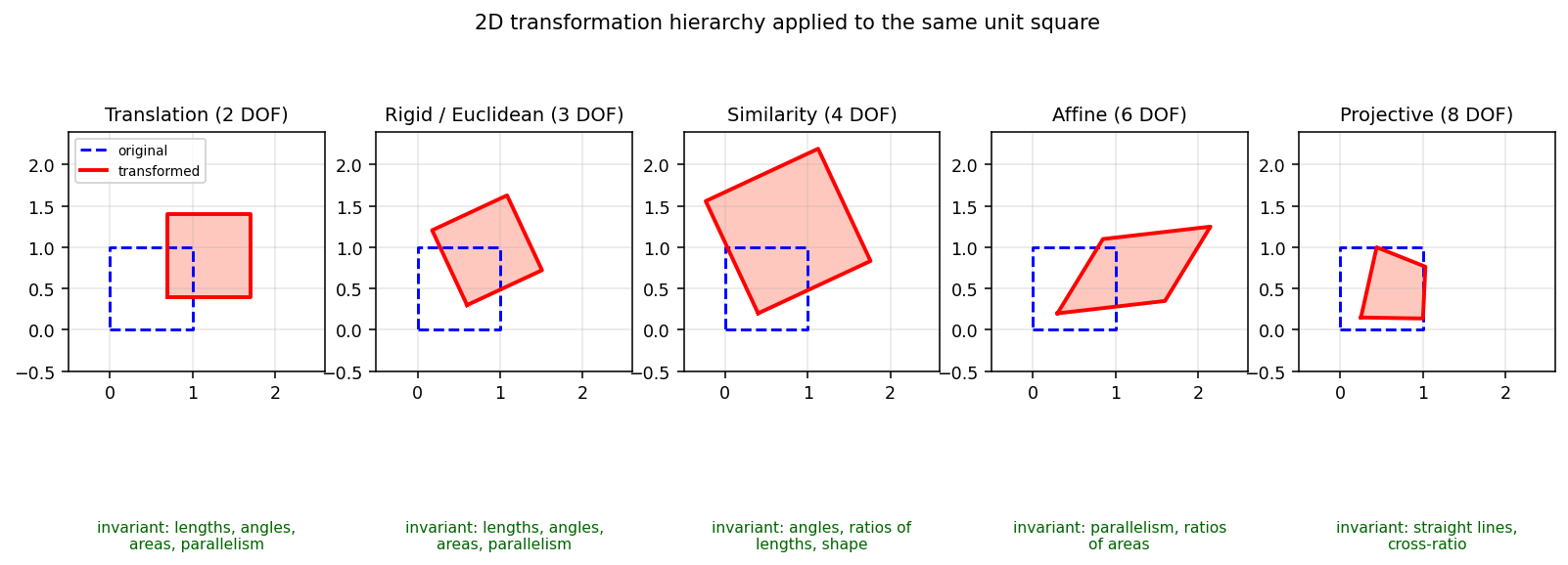
The same unit square under the five transformation families: translation (2 DOF), rigid (3), similarity (4), affine (6), projective (8) — with each family's invariants listed underneath. বাংলা: একই unit square পাঁচ পরিবারের হাতে: translation (2 DOF), rigid (3), similarity (4), affine (6), projective (8) — নিচে প্রতিটার invariant লেখা।
Read the figure left to right as "freedom increasing, invariants dissolving": the square survives as a square until similarity, becomes a parallelogram at affine, and a general quadrilateral at projective. If an exam question shows a distorted square, classify it by what is still true: parallel sides → at most affine; equal angles → at most similarity.
বাংলা: ছবিটা বাঁ থেকে ডানে পড়ুন: স্বাধীনতা বাড়ছে, invariant গলে যাচ্ছে। পরীক্ষায় বিকৃত চতুর্ভুজ দেখালে উল্টো প্রশ্ন করুন — "কোন ধর্মটা এখনো টিকে আছে?" বাহুগুলো এখনো সমান্তরাল? তাহলে বড়জোর affine। কোণগুলোও সমান? তাহলে বড়জোর similarity।
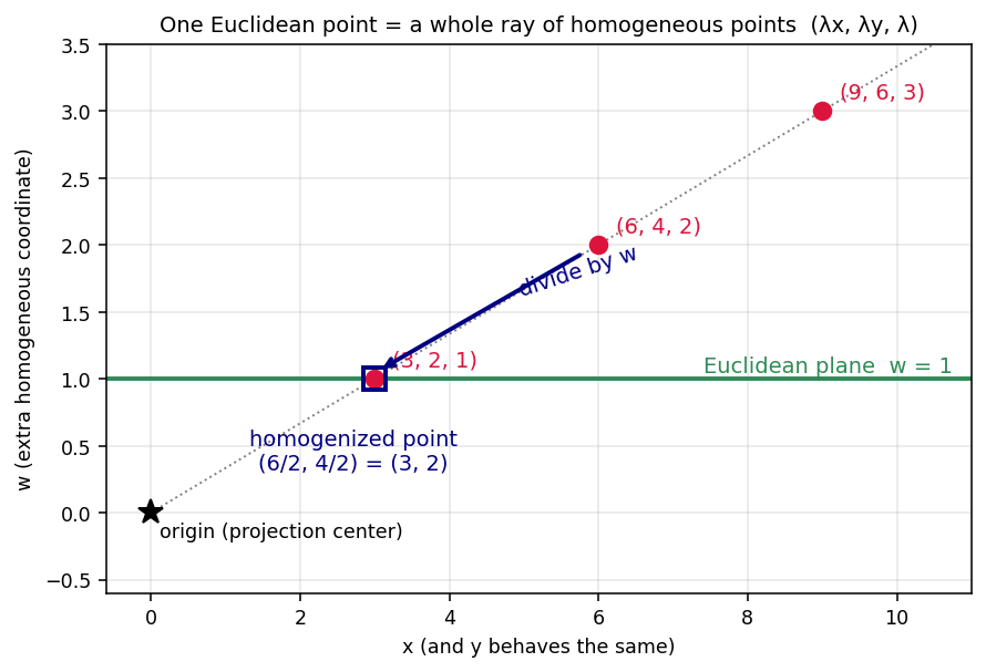
One Euclidean point is a whole ray of homogeneous representatives (6,4,2) ≡ (3,2,1) ≡ (9,6,3); homogenization divides by w and lands on the w = 1 plane at (3, 2). বাংলা: একটা Euclidean point মানে homogeneous প্রতিনিধিদের গোটা একটা ray — (6,4,2) ≡ (3,2,1) ≡ (9,6,3); w দিয়ে ভাগ করলেই w = 1 সমতলে (3,2)-তে নামা যায়।
This picture is why a homography has 8 DOF, not 9: scaling H by λ just slides results along their rays, and the division brings them back to the same spot on the w = 1 plane.
বাংলা: এই ছবিটাই homography-র 8-DOF রহস্য: H-কে λ দিয়ে গুণ করলে ফলাফল শুধু নিজের ray বরাবর সরে, w-ভাগ আবার একই জায়গায় ফিরিয়ে আনে — তাই একটা parameter অর্থহীন।
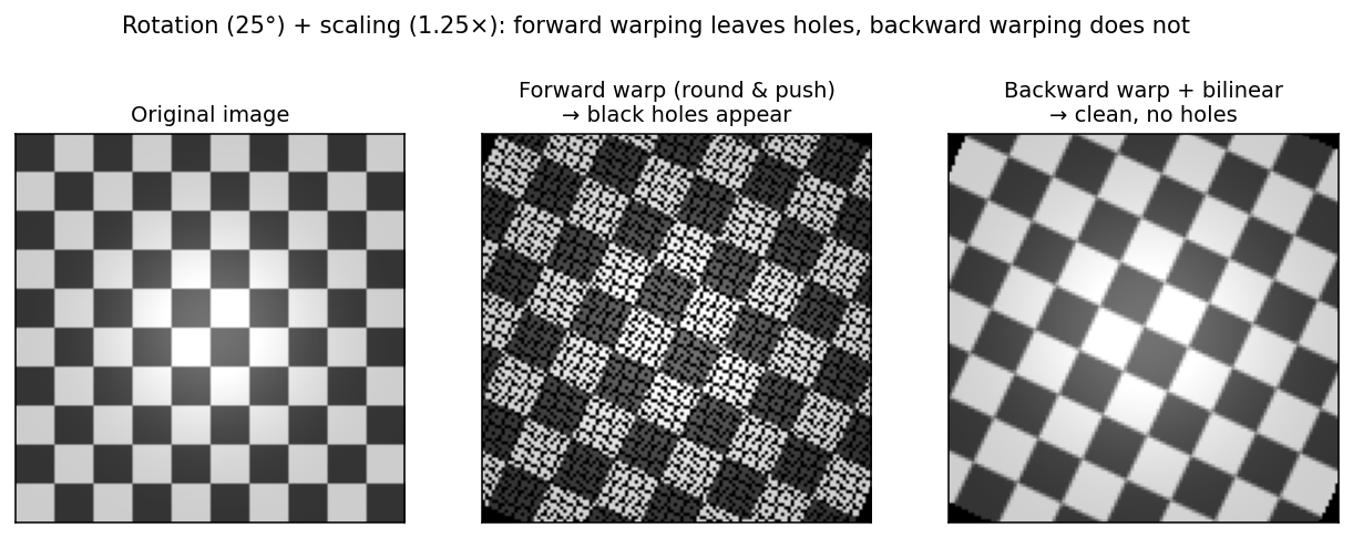
A checkerboard rotated 25° and scaled 1.25×. Forward warping (push + round) leaves black holes where no input pixel lands; backward warping (pull via T⁻¹ + bilinear interpolation) fills every output pixel. বাংলা: 25° ঘোরানো আর 1.25× বড় করা checkerboard। Forward warping (ঠেলা + rounding) কালো ফুটো রেখে যায়; backward warping (T⁻¹ দিয়ে টানা + bilinear) প্রতিটা output pixel ভরে দেয়।
The holes are not a bug in the code — they are intrinsic to pushing a discrete grid through a spreading map. Whenever a question shows a "speckled/holey" warped image, the answer keywords are: forward warping, grid misalignment, holes, fix = backward warping + interpolation.
বাংলা: ফুটোগুলো code-এর ভুল না — ছড়িয়ে-পড়া map-এর ভেতর দিয়ে discrete grid ঠেললে এটা হবেই। পরীক্ষায় "ছোপ-ছোপ ফুটোওয়ালা warped ছবি" দেখালেই keyword লিখুন: forward warping, grid-এ না পড়া, hole, সমাধান = backward + interpolation।
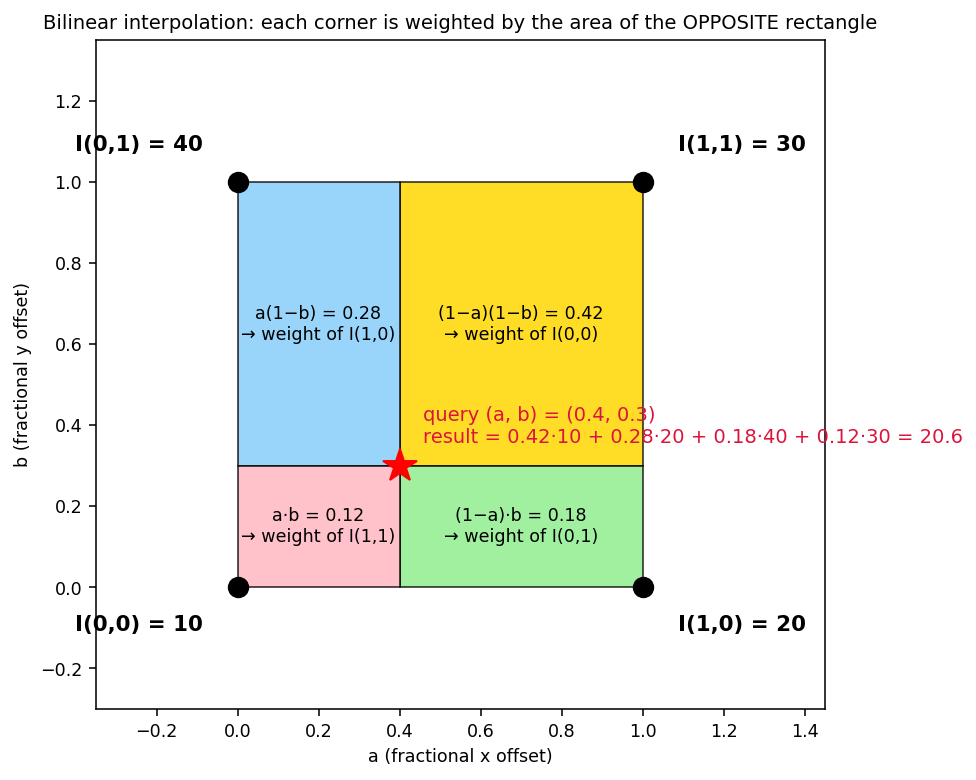
The 2×2 cell around the query (a, b) = (0.4, 0.3). Each corner's weight equals the area of the opposite colored rectangle; with corner values 10/20/40/30 the result is 0.42·10 + 0.28·20 + 0.18·40 + 0.12·30 = 20.6. বাংলা: Query (a, b) = (0.4, 0.3)-এর চারপাশের 2×2 ঘর। প্রতিটা কোণার ওজন = উল্টো দিকের রঙিন আয়তক্ষেত্রের ক্ষেত্রফল; মান 10/20/40/30 হলে ফল 20.6।
The "opposite area" rule makes the asymmetry obvious: the query sits closest to the (0,0) corner, so that corner owns the biggest rectangle (0.42). Verify the weights sum to 1 before computing — free error check.
বাংলা: "উল্টো ক্ষেত্রফল" নিয়মটা চোখে দেখালে আর ভুল হয় না: query যে কোণার কাছে, সেই কোণার ওজনই সবচেয়ে বড় (এখানে 0.42)। হিসাবের আগে ওজন চারটা যোগ করে 1 মেলান — বিনা খরচে ভুল ধরা পড়ে।
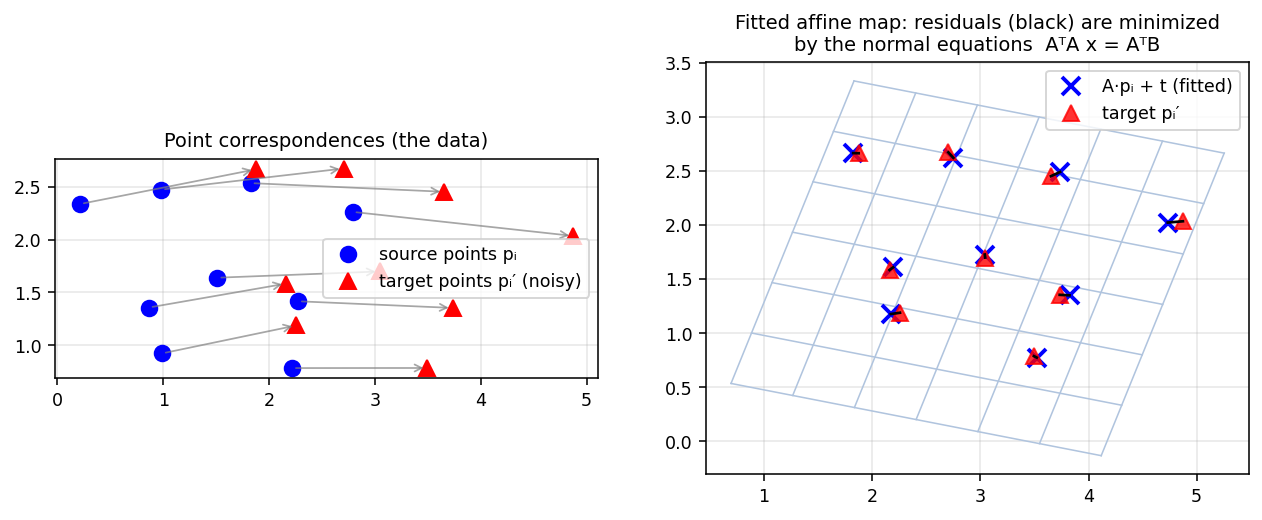
Left: noisy point correspondences (blue source → red target). Right: the affine map fitted by the normal equations A⊤Ax = A⊤b — the fitted grid, the mapped points, and the leftover residuals (black segments) that least squares has minimized. বাংলা: বাঁয়ে noisy correspondence (নীল source → লাল target)। ডানে normal equations দিয়ে fit করা affine map — warp হওয়া grid, map-করা point, আর least squares যেটা ছোট করেছে সেই অবশিষ্ট residual (কালো রেখা)।
With more than 3 correspondences and noise, no affine map hits every target — the black residual segments are the unavoidable compromise, and \(\Sigma \|residual\|^{2}\) is exactly what the normal equations minimize.
বাংলা: ৩টার বেশি noisy match থাকলে কোনো affine map-ই সব target ছুঁতে পারে না — কালো residual-গুলোই অনিবার্য আপস, আর normal equations ঠিক \(\Sigma \|residual\|^{2}\) minimize করে।
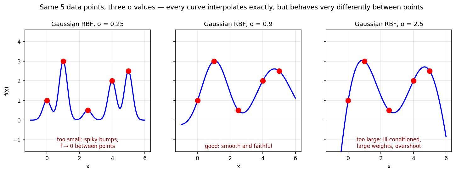
Five data points interpolated with Gaussian RBFs at σ = 0.25, 0.9, 2.5. All three curves pass exactly through the data; between the points they behave completely differently — spikes, faithful curve, oscillating overshoot. বাংলা: পাঁচটা data point, তিনটা σ-তে Gaussian RBF interpolation। তিনটা curve-ই data ঠিক ছুঁয়ে যায়; কিন্তু মাঝের আচরণ একেবারে আলাদা — কাঁটা, বিশ্বস্ত curve, দুলতে-থাকা overshoot।
Memorize the failure modes: σ too small → interpolant collapses to ~0 between sites (bumps don't overlap); σ too large → ill-conditioned Φ, giant weights of alternating sign, oscillation. "Exact at the data" says nothing about quality in between.
বাংলা: দুই ব্যর্থতার চেহারা মুখস্থ করুন: σ ছোট → মাঝখানে শূন্যে ধস (ঢিবিরা একে অন্যকে ছোঁয় না); σ বড় → Φ ill-conditioned, পালা-করে-চিহ্ন-বদলানো বিশাল weight, দোলা। "Data-তে exact" মানেই মাঝে ভালো — এমন না।
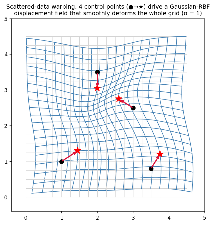
Four control points (●) dragged to new positions (★) define a scattered displacement field; Gaussian RBF interpolation (σ = 1) extends it smoothly to the entire grid — gray = original, blue = warped. বাংলা: চারটা control point (●) টেনে নতুন জায়গায় (★) নেওয়া হয়েছে; Gaussian RBF interpolation (σ = 1) সেই displacement-কে মসৃণভাবে গোটা grid-এ ছড়িয়ে দিয়েছে — ধূসর = আগের, নীল = warp হওয়া।
This is scattered-data warping in its purest form: solve two small RBF systems (one for Δx, one for Δy at the 4 controls), then evaluate everywhere. Exactly the mechanism behind landmark-driven face warps in Chapter 9.
বাংলা: এটাই scattered-data warping-এর শুদ্ধতম রূপ: ৪টা control-এ Δx আর Δy-র জন্য দুটো ছোট RBF system সমাধান, তারপর সব জায়গায় evaluate। Chapter 9-এর landmark-চালিত মুখ-warp ঠিক এই কলকব্জাতেই চলে।
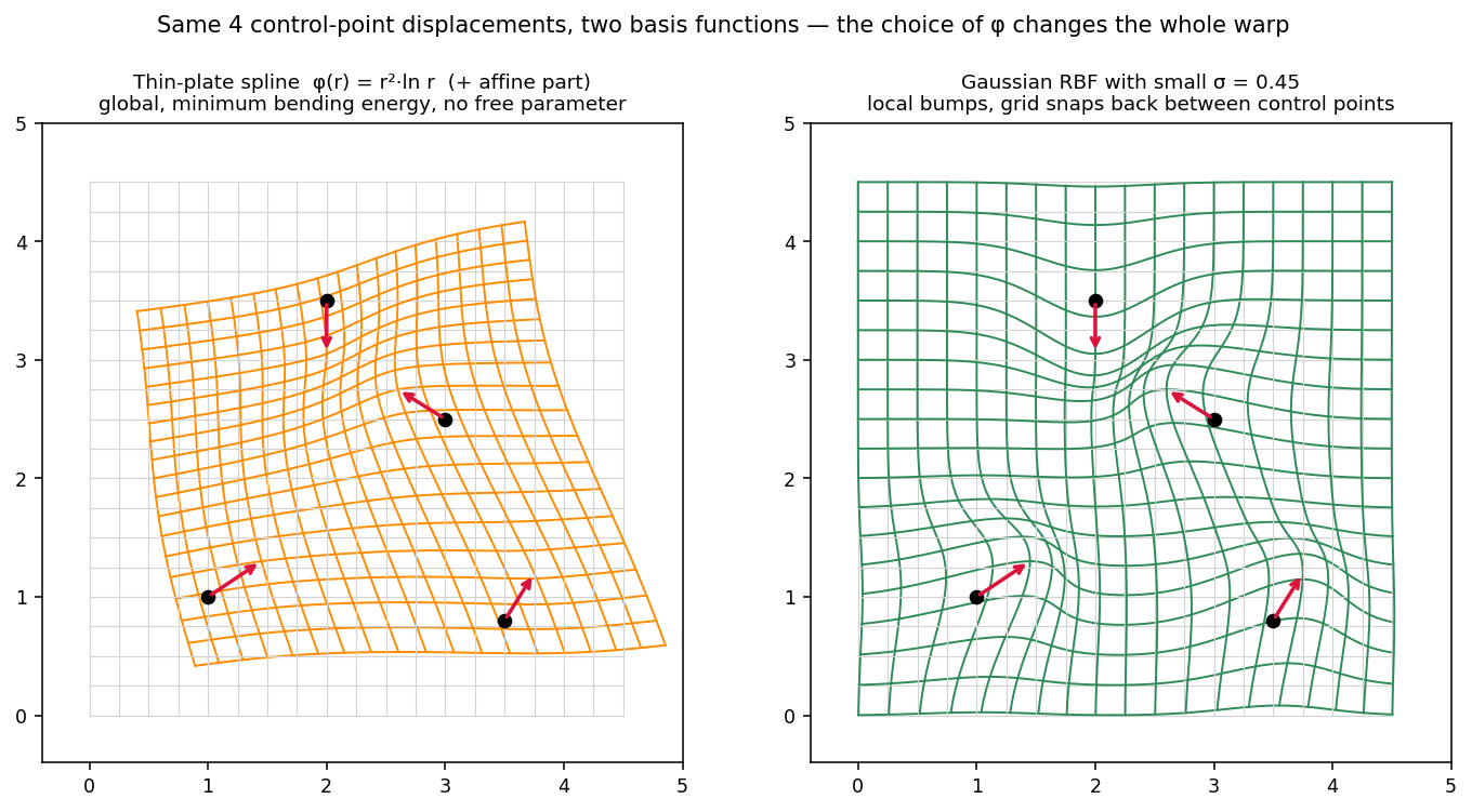
The same four control-point displacements interpolated two ways: thin-plate spline (φ = r²·ln r + affine part, parameter-free, globally smooth) versus a narrow Gaussian RBF (σ = 0.45, local bumps; the grid snaps back to identity away from the controls). বাংলা: একই চারটা control displacement দুই ভাবে interpolate করা: thin-plate spline (φ = r²·ln r + affine অংশ, parameter-free, globally মসৃণ) বনাম সরু Gaussian RBF (σ = 0.45 — স্থানীয় ঢিবি, control থেকে দূরে grid আবার আগের জায়গায় ফিরে যায়)।
The φ choice is the model: TPS distributes the bending over the whole sheet (minimum bending energy — note even far grid lines lean), while a small-σ Gaussian treats each control as a local poke. Neither is "right"; TPS wins when you want one coherent, maximally smooth deformation, local RBFs win when edits must stay local.
বাংলা: φ বেছে নেওয়াটাই model বেছে নেওয়া: TPS বাঁকানোটা গোটা পাতে ভাগ করে দেয় (minimum bending energy — দূরের grid line-ও হেলে), আর ছোট-σ Gaussian প্রতিটা control-কে স্থানীয় খোঁচা ভাবে। কোনোটা "সঠিক" নয় — এক-টানা মসৃণ বিকৃতি চাইলে TPS, সম্পাদনা স্থানীয় রাখতে চাইলে local RBF।
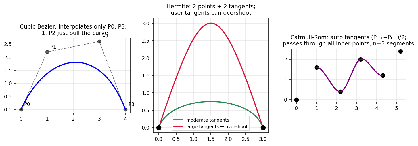
Left: cubic Bézier interpolates only P0 and P3 — P1, P2 pull. Middle: Hermite with moderate vs large tangents — large tangents overshoot. Right: Catmull-Rom passes through every inner control point using automatic tangents (Pᵢ₊₁ − Pᵢ₋₁)/2. বাংলা: বাঁয়ে cubic Bézier — শুধু P0, P3 ছোঁয়, P1, P2 টানে। মাঝে Hermite — বড় tangent দিলে overshoot। ডানে Catmull-Rom — স্বয়ংক্রিয় tangent দিয়ে প্রতিটা ভেতরের point ছুঁয়ে যায়।
The trial exam asks precisely the middle-vs-right comparison (Q6c): same cubic Hermite machinery, different tangent source — user-supplied (can overshoot) vs neighbor-derived (never needs hand-tuning, interpolates all inner points).
বাংলা: Trial exam-এর Q6c ঠিক মাঝের-বনাম-ডানের তুলনা: একই cubic Hermite যন্ত্র, tangent-এর উৎসটাই শুধু আলাদা — ব্যবহারকারীর দেওয়া (overshoot হতে পারে) বনাম প্রতিবেশী-থেকে-আসা (হাত লাগাতে হয় না, সব ভেতরের point ছোঁয়)।
§6 Algorithms & Code¶
6.1 Homogeneous toolkit: T, R, S, chaining, and rotation around a point¶
"""
Purpose:
  Build the 3×3 building blocks T, R, S, chain them into M = T·R·S,
  apply the chain to a square — the exact machinery of trial-exam Q6a/Q6b.
"""
import numpy as np

def to_h(p):   return np.hstack([p, np.ones((len(p), 1))])   # (x,y) → (x,y,1)
def from_h(q): return q[:, :2] / q[:, 2:3]                   # divide by w — ALWAYS

def T(tx, ty): return np.array([[1, 0, tx], [0, 1, ty], [0, 0, 1]], float)
def S(sx, sy): return np.array([[sx, 0, 0], [0, sy, 0], [0, 0, 1]], float)
def R(theta):
    c, s = np.cos(theta), np.sin(theta)
    return np.array([[c, -s, 0], [s, c, 0], [0, 0, 1]], float)

square = np.array([[-1, -1], [1, -1], [1, 1], [-1, 1]], float)
M = T(20, 0) @ R(np.pi / 4) @ S(2, 1)     # read right-to-left: scale, rotate, translate
warped = from_h((M @ to_h(square).T).T)

def rotate_around(P, theta, pts):         # trial-exam Q6b in one line
    M = T(P[0], P[1]) @ R(theta) @ T(-P[0], -P[1])
    return from_h((M @ to_h(pts).T).T)
Step-by-step. \(to_{h}\) lifts points to homogeneous coordinates; \(from_{h}\) divides by the last coordinate (harmless for affine where w = 1, essential for homographies). The chain \(T(20,0) @ R(\pi /4) @ S(2,1)\) is one matrix — applied once per point. rotate_around is the 3-step pattern \(T(P)\cdot R(\theta )\cdot T(-P)\) verbatim.
Exam relevance. Swap the order to S @ R @ T and plot — the result differs visibly: matrix multiplication is not commutative. State the order explicitly in every exam answer.
বাংলা: \(from_{h}\)-এর ভাগটা কখনো বাদ দেবেন না — affine-এ w = 1 বলে ক্ষতি নেই, কিন্তু homography-তে এটাই আসল কাজ। আর rotate_around মানে তিন ধাপ এক লাইনে: pivot-কে origin-এ আনো, ঘোরাও, ফেরত পাঠাও। Order বদলালে ফল বদলায় — পরীক্ষায় order লিখে দিন।
6.2 Backward warping with bilinear interpolation¶
def bilinear(I, x, y):
    """Sample image I at the fractional position (x, y) — §4.9 verbatim."""
    x0, y0 = int(np.floor(x)), int(np.floor(y))
    a, b = x - x0, y - y0
    top    = (1 - a) * I[y0,     x0] + a * I[y0,     x0 + 1]
    bottom = (1 - a) * I[y0 + 1, x0] + a * I[y0 + 1, x0 + 1]
    return (1 - b) * top + b * bottom

def backward_warp(I, M, out_shape):
    """For every OUTPUT pixel p', read the input at M⁻¹·p' — no holes."""
    Minv = np.linalg.inv(M)
    Hh, Ww = out_shape
    J = np.zeros(out_shape)
    for yo in range(Hh):
        for xo in range(Ww):
            x, y, w = Minv @ np.array([xo, yo, 1.0])
            x, y = x / w, y / w                      # homography-safe divide
            if 0 <= x < I.shape[1] - 1 and 0 <= y < I.shape[0] - 1:
                J[yo, xo] = bilinear(I, x, y)
    return J
Step-by-step. The loop runs over output pixels; Minv answers "where did this pixel come from?"; bilinear blends the 2×2 neighborhood at the fractional landing spot. Out-of-range sources stay 0 (the new black border of a rotated image). cv2.warpAffine/cv2.warpPerspective are exactly this, vectorized.
Exam relevance. Be able to write or explain this double structure: invert, loop over output, divide by w, interpolate. Forward warping = same loop over the input without the inverse — and with holes.
বাংলা: মন্ত্রটা code-এ পড়ুন: output pixel ধরে \(M^{-1}\) লাগাও → w দিয়ে ভাগ → ভগ্নাংশ জায়গায় bilinear। এতে প্রতিটা output pixel ঠিক একটা মান পায় — ফুটো অসম্ভব। cv2.warpPerspective ভেতরে ভেতরে ঠিক এটাই করে।
6.3 Least-squares affine fit from correspondences¶
def fit_affine_lsq(src, dst):
    """src, dst: (N, 2) arrays, N ≥ 3 non-collinear. Normal equations per channel (§4.7)."""
    A = np.hstack([src, np.ones((len(src), 1))])        # design-matrix rows (xᵢ, yᵢ, 1)
    px = np.linalg.solve(A.T @ A, A.T @ dst[:, 0])      # (a11, a12, tx)
    py = np.linalg.solve(A.T @ A, A.T @ dst[:, 1])      # (a21, a22, ty)
    return np.vstack([px, py, [0, 0, 1]])
Step-by-step. One design matrix A serves both channels; the two solve calls are the normal equations \(A^{\top}A\cdot x = A^{\top}b\) for the x'-targets and the y'-targets. With exactly 3 non-collinear points the residual is zero; with more (noisy) points you get the least-squares compromise from the §5 figure.
Exam relevance. This is the hand-computation of §4.7/C11 mechanized — know both directions.
বাংলা: A একটাই, target দুটো — x'-এর জন্য এক সমাধান, y'-এর জন্য আরেক। ৩টা ভালো point-এ residual শূন্য; বেশি noisy point-এ least squares সেরা আপস বেছে নেয়। Collinear source point দিলে \(A^{\top}A\) singular — solve ভেঙে পড়বে, পরীক্ষাতেও সেটাই উত্তর।
6.4 Homography by DLT (recovered exercise code)¶
def homography_dlt(src, dst):
    """≥ 4 correspondences, no 3 collinear → H with H[2,2] = 1."""
    A = []
    for (x, y), (xp, yp) in zip(src, dst):
        A.append([-x, -y, -1,  0,  0,  0, x * xp, y * xp, xp])
        A.append([ 0,  0,  0, -x, -y, -1, x * yp, y * yp, yp])
    _, _, Vt = np.linalg.svd(np.array(A))
    H = Vt[-1].reshape(3, 3)        # right-singular vector of the smallest singular value
    return H / H[2, 2]
Step-by-step. Each correspondence contributes 2 rows of the 2N×9 system \(A\cdot h = 0\); the SVD's last right-singular vector is the unit-norm h minimizing \(\|A\cdot h\|^{2}\) — least squares again, just in homogeneous disguise. Normalizing by H[2,2] fixes the free scale (the "9 − 1 = 8 DOF" convention). One-liners in practice: cv2.findHomography(src, dst, cv2.RANSAC) to estimate (outlier-robust, see §8 D17), cv2.warpPerspective(img, H, dsize) to apply with backward warping.
বাংলা: প্রতি match-এ ২টা সারি, ৪ match-এ 8×9 system; SVD-র সবচেয়ে ছোট singular value-র vector-টাই h। শেষে H[2,2] দিয়ে ভাগ — ওটাই "free scale" parameter মেরে ফেলা। বাস্তবে এক লাইনে: cv2.findHomography(..., cv2.RANSAC)।
6.5 Gaussian RBF scattered-data interpolation¶
def rbf_fit(xs, ys, sigma):
    """Solve Φ·w = y for 1-D sites xs and values ys (§4.11)."""
    Phi = np.exp(-(xs[:, None] - xs[None, :]) ** 2 / (2 * sigma ** 2))
    return np.linalg.solve(Phi, ys)

def rbf_eval(xq, xs, w, sigma):
    Pq = np.exp(-(xq[:, None] - xs[None, :]) ** 2 / (2 * sigma ** 2))
    return Pq @ w
Step-by-step. \(Phi[j, i] = \phi (|x_{j} - x_{i}|)\) with diagonal 1; solve gives the weights; evaluation is the weighted bump sum \(f(x) = \Sigma w_{i}\cdot \phi (|x - x_{i}|)\). For a 2-D image warp, run this twice on the control points — once with the Δx displacements as ys, once with Δy — exactly what produced the §5 grid-warp figure (with squared 2-D distances inside the exponential).
বাংলা: তিন লাইনের রেসিপি: দূরত্ব → Φ, solve → w, ঢিবির যোগফল → f। ছবির warp-এ control point-গুলোর Δx আর Δy আলাদা দুটো একই রকম সমস্যা। σ ছোট/বড় করলে কী হয় — §4.10 আর §5-এর তিন-প্যানেল ছবিটা মনে করুন।
6.6 Bézier and Catmull-Rom segments (recovered exercise code)¶
def bezier3(P0, P1, P2, P3, n=100):
    """Cubic Bézier — Bernstein weights, interpolates only P0 and P3."""
    t = np.linspace(0, 1, n)[:, None]
    return ((1 - t) ** 3) * P0 + 3 * (1 - t) ** 2 * t * P1 \
         + 3 * (1 - t) * t ** 2 * P2 + t ** 3 * P3

def catmull_rom(P0, P1, P2, P3, n=50):
    """One C-R segment from P1 to P2; P0, P3 only shape the auto-tangents."""
    t = np.linspace(0, 1, n)[:, None]
    a = -0.5 * P0 + 1.5 * P1 - 1.5 * P2 + 0.5 * P3
    b =        P0 - 2.5 * P1 + 2.0 * P2 - 0.5 * P3
    c = -0.5 * P0             + 0.5 * P2
    d =                  P1
    return ((a * t + b) * t + c) * t + d
Step-by-step. bezier3 is the Bernstein form of §4.13 (check: at t = 0.5 with the §4.13 control points it returns (2.0, 1.875)). catmull_rom is the Hermite basis with the auto-tangents \((P_{i+1} - P_{i-1})/2\) already multiplied through into polynomial coefficients a, b, c, d — at t = 0 it returns P1, at t = 1 it returns P2. Chain segments over a sliding window of 4 points for a full curve (n points → n − 3 segments).
বাংলা: bezier3-তে চারটা weight-এর যোগফল সব t-তে 1 — তাই curve convex hull ছাড়ে না। catmull_rom-এ tangent আগে থেকেই coefficient-এ গোঁজা; t=0-তে P1, t=1-এ P2 — ভেতরের point সবসময় ছোঁয়। পুরো curve মানে ৪-point জানালা সরিয়ে সরিয়ে segment জোড়া।
6.7 Thin-plate spline solve and apply (recovered exercise code)¶
def tps_solve(src, dst):
    """src, dst: (n, 2). Returns n RBF weights + 3 affine rows per output dim."""
    n = len(src)
    K = np.zeros((n, n))
    for i in range(n):
        for j in range(n):
            r2 = ((src[i] - src[j]) ** 2).sum()
            K[i, j] = r2 * np.log(r2 + 1e-12)       # = 2·r²·ln r (φ up to a constant)
    P = np.hstack([np.ones((n, 1)), src])
    L = np.zeros((n + 3, n + 3))
    L[:n, :n] = K;  L[:n, n:] = P;  L[n:, :n] = P.T
    Y = np.zeros((n + 3, 2));  Y[:n] = dst
    return np.linalg.solve(L, Y)

def tps_apply(params, src, x):
    n = len(src)
    w, A = params[:n], params[n:].T                 # RBF weights, 2×3 affine part
    out = np.hstack([np.ones((len(x), 1)), x]) @ A.T
    for i, p in enumerate(src):
        r2 = ((x - p) ** 2).sum(axis=1)
        out += w[i] * (r2 * np.log(r2 + 1e-12))[:, None]
    return out
Step-by-step. L stacks the §4.14 structure: N interpolation rows [K | P] plus 3 constraint rows \([P^{\top} | 0]\) — the constraints \(\Sigma w_{i} = 0, \Sigma w_{i}x_{i} = 0, \Sigma w_{i}y_{i} = 0\) enter as the bottom block equaling zero. Implementation tricks: \(r^{2}\cdot \ln (r^{2}) = 2\cdot r^{2}\cdot \ln r\) is the TPS kernel up to a factor 2 that the weights absorb (and avoids a square root); +1e-12 dodges ln 0 at r = 0 where φ → 0 anyway. tps_apply evaluates affine part + bump sum; solving \(Y[:n] = dst\) handles both output coordinates in one go.
Exam relevance. You will not reproduce this from memory — but recognize the (n+3)×(n+3) structure, the kernel, and the role of the 3 constraint rows.
বাংলা: Matrix L-এর চেহারাটাই গল্পটা: উপরে N সারি "প্রতিটা নাট-বল্টু ছুঁতে হবে", নিচে ৩ সারি "affine-সাধ্য কাজ RBF নেবে না"। \(r^{2}\cdot \ln (r^{2})\) লেখা মানে φ-এর দ্বিগুণ — ওই 2 weight-এর ভেতরে মিশে যায়। আর 1e-12 শুধু ln 0-এর crash ঠেকায়।
§7 Trial-Exam Mapping¶
| Trial-exam item | What you must know | Where in this chapter |
|---|---|---|
| Q6a Decompose \(M = [[0,-1,0],[1,0,20],[0,0,1]]\) into T·R·S | Read-off rules: last column → \(t = (0, 20)\); column lengths of the 2×2 block → \(s_{x} = s_{y} = 1\); \(\alpha = \operatorname{atan2}(1, 0) = 90^{\circ}\) (the hint \(\operatorname{atan2}(1,0) = \pi /2\) was printed on the exam) | §4.4, worked twice |
| Q6b Rotate a shape around a specific point P | The 3-step pattern: translate by −P, rotate by θ, translate back by +P, i.e. \(M = T(P)\cdot R(\theta )\cdot T(-P)\) | §4.4, §6.1 |
| Q6c Catmull-Rom vs Hermite splines | Same cubic Hermite basis; difference = tangent source: Hermite = user-supplied (overshoot risk), Catmull-Rom = automatic \((P_{i+1} - P_{i-1})/2\), interpolates every inner point, n points → n−3 segments | §4.13, §5 spline figure |
Model answer (Q6b): "Rotation matrices rotate around the origin. To rotate around P instead: (1) translate the scene by −P so that P moves to the origin, (2) apply R(θ), (3) translate back by +P. Combined: M = T(P)·R(θ)·T(−P), read right to left."
Model answer (Q6c): "Both are cubic splines built on the Hermite basis. A Hermite spline needs two endpoints plus two user-supplied tangent vectors per segment — flexible, but large tangents overshoot. A Catmull-Rom spline computes the tangents automatically from the neighboring control points, Pᵢ' = (Pᵢ₊₁ − Pᵢ₋₁)/2, so it interpolates every inner control point with C¹-continuous joints and needs no manual tuning."
The fully graded answers are in CVML_Trial_Exam_Analysis.md.
§8 Mock Exam — 20 Questions¶
Answer everything on paper first; full worked solutions follow in §8.5. Tier A = basics, B = intuition, C = harder computation/derivation, D = transfer questions slightly beyond the lecture (typical for a tough oral or a "Transfer" section in the written exam).
Tier A — Basic (definitions & direct formula use)¶
A1. State the degrees of freedom of the five 2-D transformation families (translation, rigid, similarity, affine, projective) and the minimum number of point correspondences needed to estimate each.
A2. Rotate the point \(p = (3, 4)\) by 90° around the origin. Write down R(90°), compute p', and verify with a length check.
A3. (a) Which 2-D point does the homogeneous vector (9, 6, 3) represent? (b) Give two other homogeneous representatives of the same point. © Translate the original vector by \(t = (2, -1)\) in homogeneous form and homogenize the result.
A4. A shape is scaled by 2 (uniformly), then rotated by 90°, then translated by (5, 1) — in that order, column-vector convention. Write the three matrices, state the order of the product, and compute the single combined 3×3 matrix.
A5. Fill the gaps: "An affine transformation preserves ______ and ratios of ______; a circle becomes an ______ and a square becomes a ______. A projective transformation only preserves ______ and the ______; parallel lines may meet in a ______ point."
Tier B — Intuitive (why / when)¶
B6. Why does forward warping produce holes in the output image, why does backward warping not, and which two extra ingredients does backward warping need to work?
B7. Why can translation not be written as a 2×2 matrix acting on (x, y), and how exactly do homogeneous coordinates fix this? What additional famous transformation family do the same coordinates unlock?
B8. A homography matrix has 9 entries. Explain carefully why it has only 8 degrees of freedom, and connect this number to the minimum count of point correspondences.
B9. Describe the behavior of a Gaussian-RBF interpolant when σ is (a) much smaller than the data spacing, (b) much larger, © about right — and explain why the linear system becomes ill-conditioned in case (b).
B10. In the RBF model \(f(x) = \Sigma w_{i}\cdot \phi (\|x - x_{i}\|)\), why are the weights wᵢ generally not equal to the data values yᵢ? In which limit do they become (approximately) equal?
Tier C — Harder (multi-step computation / derivation)¶
C11. Fit an affine transform by least squares to the three correspondences \((0,0)\to (2,1)\), \((1,0)\to (4,2)\), \((0,1)\to (3,3)\): build the design matrix, write the normal equations \(A^{\top}A\cdot x = A^{\top}b\) for both channels, solve them by hand, and verify on two of the points.
C12. Apply the homography \(H = [[2, 0, 1], [0, 2, 0], [1, 0, 2]]\) to the points \(p = (1, 1)\) and \(q = (3, 1)\) — including the divide-by-w step. Both inputs share y = 1; explain why the outputs do not share their y value.
C13. Decompose \(M = [[\sqrt{3}, -1, 4], [1, \sqrt{3}, -2], [0, 0, 1]]\) into T·R·S using the read-off rules, and verify by multiplying back the 2×2 block.
C14. A 1-D Gaussian RBF interpolant (σ = 1) must satisfy \(f(0) = 2\) and \(f(1) = 1\). Set up Φ, solve \(\Phi w = y\) by hand (4 decimals), verify both interpolation conditions, and comment on the sign of w₂.
C15. Rotate the point \(p = (5, 2)\) by 90° around the pivot \(P = (3, 3)\) using the 3-step method; then compute the single combined matrix \(M = T(P)\cdot R(90^{\circ})\cdot T(-P)\) and confirm it sends p to the same place. Add a distance-to-pivot sanity check.
Tier D — Transfer (adjacent to, but beyond, the lecture)¶
D16. Thin-plate spline vs Gaussian RBF for warping: compare the kernels (\(r^{2}\cdot \ln r\) vs \(\exp (-r^{2}/2\sigma ^{2})\)) regarding free parameters, locality of influence, behavior far from the control points, and the optimality property TPS has. Evaluate φ_TPS at r = 0.5, 1, and e, and explain what the sign pattern tells you. Which would you pick for (i) face morphing with 60 landmarks, (ii) a local "liquify" brush edit?
D17. You estimate a homography from 100 SIFT matches of which ~30% are wrong (outliers). (a) Why does plain least squares / DLT fail badly here? (b) Sketch the RANSAC loop for this problem. © Compute how many RANSAC iterations guarantee, with 99% confidence, at least one all-inlier sample (inlier ratio w = 0.7, sample size s = 4). (d) Why is the final model still refit with least squares?
D18. Image stitching: a colleague uses an affine transform to align two photos of a large flat wall taken with strong camera rotation, and the mosaic shows ghosting toward the edges. (a) Which 2 DOF is the affine model missing and what is their geometric job? (b) Why does the error grow toward the image borders? © Name two imaging situations where the affine model would have been good enough.
D19. Shepard/IDW with \(p = 2\) on the 1-D data \((x_{1}, y_{1}) = (0, 4)\) and \((x_{2}, y_{2}) = (2, 0)\): (a) compute f(0.5); (b) compare with linear interpolation; © what does f converge to as \(p \to \infty\), and (d) what value does f approach very far from both data points? (e) Name the two structural artifacts that make IDW surfaces look characteristic.
D20. Bicubic vs bilinear interpolation: compare neighborhood size, smoothness, and sharpness. Then show with the 1-D samples \(f(-1) = 0, f(0) = 0, f(1) = 0, f(2) = 40\) and the Catmull-Rom weights at t = 0.5, namely \((-1/16, 9/16, 9/16, -1/16)\), that cubic interpolation can undershoot the data range — and explain why bilinear provably never can.
§8.5 Solutions¶
Tier A¶
A1.
| Family | DOF | Min. correspondences |
|---|---|---|
| Translation | 2 | 1 |
| Rigid / Euclidean | 3 | 2 |
| Similarity | 4 | 2 |
| Affine | 6 | 3 (not collinear) |
| Projective / homography | 8 | 4 (no 3 collinear) |
Rule: each correspondence yields 2 scalar equations, so you need ⌈DOF/2⌉ of them. বাংলা: DOF সিঁড়ি 2-3-4-6-8 আর correspondence 1-2-2-3-4 — দুটোই "প্রতি জোড়ায় ২ সমীকরণ" নিয়ম থেকে।
A2.
R(90°) = ⎡0 −1⎤      p' = (0·3 − 1·4, 1·3 + 0·4) = (−4, 3)
         ⎣1  0⎦
Check: ‖p‖ = √(9+16) = 5 ,  ‖p'‖ = √(16+9) = 5  ✓ (rotation preserves length)
বাংলা: R(90°) মুখস্থ: [[0,−1],[1,0]] — (x, y) যায় (−y, x)-এ। দৈর্ঘ্য check পরীক্ষায় ফাউ নম্বর।
A3.
(a) Divide by w = 3: \((9/3, 6/3) = (3, 2)\).
(b) Any λ-multiple, e.g. (3, 2, 1) and (6, 4, 2).
© \(T(2,-1)\cdot (9, 6, 3)^{\top} = (9 + 3\cdot 2, 6 + 3\cdot (-1), 3) = (15, 3, 3) \to (5, 1)\). Sanity: \((3, 2) + (2, -1) = (5, 1)\) ✓ — translation works for any w because the last column is multiplied by w.
বাংলা: Homogeneous vector দেখলেই আগে w দিয়ে ভাগ; আর λ-গুণিতক সব একই point। Translate করার পরেও ভাগটা ভুলবেন না।
A4.
S(2,2) = ⎡2 0 0⎤   R(90°) = ⎡0 −1 0⎤   T(5,1) = ⎡1 0 5⎤
         ⎢0 2 0⎥            ⎢1  0 0⎥            ⎢0 1 1⎥
         ⎣0 0 1⎦            ⎣0  0 1⎦            ⎣0 0 1⎦

Order: M = T(5,1)·R(90°)·S(2,2)   (first operation sits closest to the vector)

R·S = ⎡0 −2 0⎤        M = T·(R·S) = ⎡0 −2 5⎤
      ⎢2  0 0⎥                      ⎢2  0 1⎥
      ⎣0  0 1⎦                      ⎣0  0 1⎦
বাংলা: "আগে scale, পরে rotate, শেষে translate" মানেই matrix-এ উল্টো ক্রম: T·R·S — সবচেয়ে আগের কাজ vector-এর গা ঘেঁষে।
A5. "An affine transformation preserves parallelism and ratios of areas (also ratios of lengths on parallel lines); a circle becomes an ellipse and a square becomes a parallelogram. A projective transformation only preserves straight lines (collinearity) and the cross-ratio; parallel lines may meet in a vanishing point." বাংলা: Invariant-উল্টো-সিঁড়ি: affine-এ সমান্তরালতা বাঁচে, projective-এ শুধু "সোজা থাকে সোজা" আর cross-ratio।
Tier B¶
B6. Forward warping pushes each input pixel to \(T\cdot p\) and rounds; an expanding map spreads the inputs apart, so some output pixels are never hit — holes (and a shrinking map causes collisions, several inputs landing on one output). Backward warping loops over output pixels and asks each one where it came from (\(T^{-1}\cdot p'\)), so every output pixel receives exactly one value — holes are structurally impossible. The two ingredients it needs: (1) the inverse transformation T⁻¹, (2) interpolation (e.g. bilinear) because the source position is fractional. বাংলা: Forward = ঠেলা → ফাঁক পড়ে; backward = প্রতিটা output নিজের উৎস খোঁজে → ফাঁক অসম্ভব। লাগবে শুধু T⁻¹ আর bilinear।
B7. A 2×2 matrix gives \(x' = a\cdot x + b\cdot y\) — there is no slot for a constant, and every linear map fixes the origin, while a translation must move it. Appending a 1 creates that slot: the 3×3 matrix's last column is multiplied by the constant 1 and enters the result as \(+t_{x}, +t_{y}\). The same machinery (a non-trivial last row plus the divide-by-w) unlocks the projective transformations/homographies — perspective itself. বাংলা: Linear map origin নাড়াতে পারে না, তাই vector-এ 1 জুড়ে constant-এর জায়গা বানাই। Bonus: ওই একই কৌশলে নিচের সারি খুলে দিলেই perspective।
B8. For any λ ≠ 0, \((\lambda H)\tilde{p} = \lambda (H\tilde{p})\), and the homogenization divides the λ out again: H and λH define the identical point mapping. So one of the 9 entries is pure redundancy — fix it by \(h_{33} = 1\) (or \(\|h\| = 1\)), leaving 8 genuine parameters. Each correspondence gives 2 independent equations, hence \(8/2 = 4\) correspondences minimum (no 3 collinear). বাংলা: λH আর H ভাগের পরে এক — তাই 9 − 1 = 8 DOF, আর 8/2 = 4 match। এই দুই সংখ্যা এক সুতোয় বাঁধা।
B9. (a) σ ≪ spacing: the bumps don't overlap; Φ ≈ I, so wᵢ ≈ yᵢ, and f collapses toward 0 between the sites — a row of isolated spikes. (b) σ ≫ spacing: every entry of Φ approaches 1, the rows become nearly identical, det(Φ) → 0 — ill-conditioned: the weights must be huge and of alternating sign for the tiny row differences to reproduce the data, and the interpolant oscillates/overshoots; numerically, tiny data noise explodes into wild weight changes. © σ ≈ typical spacing: bumps overlap moderately — a smooth, faithful interpolant. বাংলা: ছোট σ = কাঁটা, বড় σ = প্রায়-singular Φ আর দুলুনি, মাঝারি σ = ঠিকঠাক। Ill-condition-এর কারণ: সারিগুলো প্রায় এক হয়ে গেলে সমাধান চরম স্পর্শকাতর হয়ে যায়।
B10. At a data site xⱼ the neighboring bumps also contribute: \(f(x_{j}) = w_{j}\cdot \phi (0) + \Sigma _{i}\neq _{j} w_{i}\cdot \phi (\|x_{j}-x_{i}\|)\). To hit yⱼ exactly, wⱼ must compensate for the neighbors' spill-over — that coupling is exactly the off-diagonal of Φ, and untangling it is why we solve \(\Phi w = y\). The weights approach the data values when the off-diagonals vanish: σ → 0, or data sites very far apart relative to σ (Φ → I). বাংলা: প্রতিবেশীর ঢিবি data point-এ উঁকি দেয় বলেই w ≠ y; সেই উঁকি-ভাগ বাদ দিতেই linear system। ঢিবিরা একে অন্যকে না ছুঁলে (σ→0) তবেই w ≈ y।
Tier C¶
C11. Design matrix rows \((x_{i}, y_{i}, 1)\); both channels share A:
A = ⎡0 0 1⎤        A⊤A = ⎡1 0 1⎤
    ⎢1 0 1⎥              ⎢0 1 1⎥
    ⎣0 1 1⎦              ⎣1 1 3⎦

x-channel, b = (2, 4, 3)⊤:  A⊤b = (4, 3, 9)⊤
   a₁₁ + t_x = 4 ;  a₁₂ + t_x = 3 ;  a₁₁ + a₁₂ + 3t_x = 9
   (4 − t_x) + (3 − t_x) + 3t_x = 9  ⟹  7 + t_x = 9  ⟹  t_x = 2, a₁₁ = 2, a₁₂ = 1

y-channel, b = (1, 2, 3)⊤:  A⊤b = (2, 3, 6)⊤
   a₂₁ + t_y = 2 ;  a₂₂ + t_y = 3 ;  a₂₁ + a₂₂ + 3t_y = 6
   (2 − t_y) + (3 − t_y) + 3t_y = 6  ⟹  5 + t_y = 6  ⟹  t_y = 1, a₂₁ = 1, a₂₂ = 2

Result:  A_affine = ⎡2 1⎤ ,  t = (2, 1)⊤
                    ⎣1 2⎦
Check (1,0): (2·1 + 1·0 + 2, 1·1 + 2·0 + 1) = (4, 2) ✓
Check (0,1): (2·0 + 1·1 + 2, 1·0 + 2·1 + 1) = (3, 3) ✓   (and (0,0) → (2,1) ✓)
With 3 exact points the residual is zero; the identical normal equations handle any larger noisy set. বাংলা: এক A, দুই channel — x'-target আর y'-target আলাদা b। তিনটা সমীকরণে substitution-এই উত্তর বেরোয়; শেষে দুটো point-এ check করলে নম্বর নিরাপদ।
C12.
Both inputs had y = 1, but \(\tilde{w}' = x + 2\) grows with x: the farther point q is divided by a larger w̃' and its y-coordinate is squeezed harder (0.4 < 0.667). That per-point division is perspective foreshortening — an affine map (w̃' ≡ 1) can never separate the two. বাংলা: নিচের সারি (1, 0, 2) মানে w̃' = x + 2 — point যত ডানে, ভাগ তত বড়, ছবি তত "চাপা"। এটাই perspective; ভাগটা ভুললে পুরো প্রশ্ন ভুল।
C13.
t = (m₁₃, m₂₃) = (4, −2)
s_x = √((√3)² + 1²) = √4 = 2 ,    s_y = √((−1)² + (√3)²) = √4 = 2
α  = atan2(m₂₁, m₁₁) = atan2(1, √3) = 30°

Verify the 2×2 block:  R(30°)·S(2,2) = ⎡cos30° −sin30°⎤·⎡2 0⎤ = ⎡√3 −1⎤ ✓
                                       ⎣sin30°  cos30°⎦ ⎣0 2⎦   ⎣1  √3⎦
⟹  M = T(4,−2) · R(30°) · S(2,2)
বাংলা: তিন নিয়ম তিন লাইনে: শেষ column → t, column-দৈর্ঘ্য → s, atan2 → α। √3-ওয়ালা matrix দেখলেই 30°/60° সন্দেহ করুন।
C14.
φ(0) = 1 ,  φ(1) = exp(−1²/(2·1²)) = e^(−0.5) = 0.6065

Φ = ⎡1      0.6065⎤ ,   y = ⎡2⎤
    ⎣0.6065 1     ⎦         ⎣1⎦

det(Φ) = 1 − 0.6065² = 1 − 0.3679 = 0.6321
w₁ = (2 − 0.6065·1)/0.6321 = 1.3935/0.6321 = 2.2045
w₂ = (1 − 0.6065·2)/0.6321 = −0.2131/0.6321 = −0.3371

Verify:  f(0) = 2.2045·1 + (−0.3371)·0.6065 = 2.2045 − 0.2045 = 2.0000 ✓
         f(1) = 2.2045·0.6065 + (−0.3371)·1 = 1.3370 − 0.3371 = 0.9999 ≈ 1 ✓
w₂ is negative: site 1's wide bump already delivers 1.337 at x = 1, more than the required y₂ = 1, so the second bump must pull down. Negative weights are perfectly normal — more evidence that weights ≠ data values. বাংলা: Cramer-এ ২ লাইনে সমাধান, তারপর দুই data point-এ verify। w₂ ঋণাত্মক — প্রতিবেশীর ঢিবি বেশি দিয়ে ফেলেছে, তাই টেনে নামাতে হচ্ছে; এতে ভয়ের কিছু নেই।
C15.
3-step:  p − P = (5−3, 2−3) = (2, −1)
         rotate 90°: (0·2 − 1·(−1), 1·2 + 0·(−1)) = (1, 2)
         + P:        (1+3, 2+3) = (4, 5)

Combined matrix:  R(90°)·T(−3,−3) has translation R·(−3,−3)⊤ = (3, −3)
                  then T(3,3) adds (3,3):  t_M = (6, 0)
M = ⎡0 −1 6⎤        M·(5, 2, 1)⊤ = (0·5 − 1·2 + 6, 1·5 + 0·2 + 0, 1) = (4, 5, 1) ✓
    ⎢1  0 0⎥
    ⎣0  0 1⎦
Sanity: ‖p − P‖ = √(4+1) = √5 ;  ‖(4,5) − (3,3)‖ = ‖(1,2)‖ = √5 ✓
বাংলা: তিন ধাপে হাতে আর এক matrix-এ যন্ত্রে — দুটোই (4,5)। Pivot থেকে দূরত্ব আগে-পরে √5: rotation দূরত্ব বদলায় না, তাই হিসাব সঠিক।
Tier D¶
D16. Kernels. Gaussian \(\exp (-r^{2}/2\sigma ^{2})\): a positive, exponentially decaying bump — influence is effectively local, far from all controls the displacement returns to ~0, and σ is a free parameter you must tune. TPS \(\phi (r) = r^{2}\cdot \ln r\): parameter-free, grows with distance — every control point influences the entire image (global), and the warp far away is governed by the affine part. TPS's unique selling point: among all interpolants it minimizes the bending energy \(\int \int f^{2}_{xx} + 2f^{2}_{xg} + f^{2}_{gg}\) — the provably smoothest solution. Values. \(\phi (0.5) = 0.25\cdot \ln 0.5 = 0.25\cdot (-0.6931) = -0.173\); \(\phi (1) = 1\cdot \ln 1 = 0\); \(\phi (e) = e^{2}\cdot 1 \approx 7.389\). Negative inside r < 1, zero at r = 1, growing without bound beyond — this is not a bump at all, which is exactly why TPS behaves globally and needs the affine part + constraints to stay well-posed. Choices. (i) Face morphing with 60 landmarks: TPS — one coherent, maximally smooth warp, nothing to tune. (ii) Liquify brush: Gaussian RBF with small σ — the edit must stay local; TPS would lean the whole image. বাংলা: Gaussian = স্থানীয় ঢিবি + σ বাছতে হয়; TPS = parameter-free, global, আর "সবচেয়ে মসৃণ" — bending energy-র গাণিতিক চ্যাম্পিয়ন। মুখ-morph-এ TPS, স্থানীয় brush-এ ছোট-σ Gaussian।
D17. (a) Least squares squares the residuals, so the ~30 gross outliers dominate the cost; a single bad match can drag H arbitrarily far (LSQ's breakdown point is 0%). The fitted homography lands "between" the true motion and the garbage. (b) RANSAC: repeat N times → randomly pick a minimal sample of s = 4 matches → fit an exact H by DLT → count inliers (matches whose transfer error \(\|p' - hom(H\cdot p)\|\) — with the divide-by-w! — is below a threshold, e.g. 1–3 px) → keep the H with the largest inlier count. © \(N \ge \log (1-p)/\log (1-w^{s})\) with p = 0.99, w = 0.7, s = 4:
w⁴ = 0.7⁴ = 0.2401          1 − w⁴ = 0.7599
N ≥ ln(0.01)/ln(0.7599) = (−4.6052)/(−0.2746) = 16.8   →   17 iterations
(d) The winning model used only 4 matches, so it is noise-sensitive; once the ~70 inliers are identified, refitting on all inliers by least squares averages out their (now outlier-free, roughly Gaussian) noise — in that regime LSQ is the right tool again. RANSAC finds who to trust; LSQ then extracts the best model from the trusted. বাংলা: Outlier থাকলে LSQ-র বর্গ-করা cost পাগল হয়ে যায়; RANSAC ছোট ছোট ৪-match নমুনায় ভোট নেয় (এখানে মাত্র ১৭ বার যথেষ্ট), তারপর জেতা inlier-দের উপর আবার LSQ — দুই হাতিয়ারের ভাগাভাগি এটাই।
D18. (a) The affine model lacks the two projective parameters h₃₁, h₃₂ (the bottom row). Their job: make \(\tilde{w}' = h_{31}x + h_{32}y + 1\) vary across the image, producing the per-point division = perspective foreshortening; geometrically they let parallel lines converge (keystone) — the 6-DOF affine map keeps them parallel forever. (b) The fit effectively linearizes the true projective map around the image center; a rational function \((\cdot )/\tilde{w}'(x,y)\) deviates from any linear approximation more and more as you move away from the center — so misalignment (ghosting) grows toward the borders, exactly where the parallax-free wall's keystoning is strongest. © Affine is good enough when perspective variation across the overlap is negligible: e.g. telephoto / narrow field of view shots of a distant planar scene (weak perspective), flatbed-scanner-like fronto-parallel captures, aerial/satellite images of flat terrain from high altitude, or a microscope stage translating a flat specimen. বাংলা: Affine-এর নিচের সারি (0, 0, 1) — তাই keystone/converging-lines বানাতে পারে না; ভুলটা কেন্দ্র থেকে দূরে বাড়ে। দূর থেকে সরু lens-এ তোলা প্রায়-সমতল দৃশ্যে affine-ই যথেষ্ট।
D19.
(a) d₁ = 0.5, d₂ = 1.5;   w₁ = 1/0.5² = 4,   w₂ = 1/1.5² = 1/2.25 = 0.4444
    f(0.5) = (4·4 + 0.4444·0)/(4 + 0.4444) = 16/4.4444 = 3.6
(b) Linear interpolation: 4 + (0.5/2)·(0 − 4) = 4 − 1 = 3.0  → IDW (3.6) clings
    harder to the nearer value because of the squared-distance weighting.
(c) p → ∞: the nearest site's weight dominates totally → nearest-neighbor
    interpolation (piecewise constant, Voronoi cells); here f(0.5) → 4.
(d) Far from all data: all distances ≈ equal → weights ≈ equal → f → mean = (4+0)/2 = 2.
(e) The two structural artifacts: bull's-eye flat spots (the gradient vanishes at every data site, creating plateaus around each sample) and the convex-combination clamp (f is trapped in [min yᵢ, max yᵢ] everywhere — no trend extrapolation). Bonus third: global O(N) influence of every site on every query. বাংলা: IDW system সমাধান করে না বলে সস্তা, কিন্তু দাগ রেখে যায়: প্রতিটা data point-এ চ্যাপ্টা bull's-eye, আর মান কখনো data-সীমার বাইরে যায় না। p বাড়ালে nearest-neighbor, দূরে গেলে সবার গড়।
D20. Comparison. Bilinear: 2×2 = 4 neighbors, continuous but with derivative kinks at cell edges (C⁰), all weights ≥ 0 summing to 1 → mild blur, never overshoots. Bicubic: 4×4 = 16 neighbors, smoother result (C¹) and visibly sharper edges — because its kernel has negative lobes, i.e. some weights < 0 (they still sum to 1). Undershoot demo. Catmull-Rom weights at t = 0.5 are \((-1/16, 9/16, 9/16, -1/16)\):
The interpolated value −2.5 lies below the data minimum 0 (linear interpolation between f(0) = 0 and f(1) = 0 would give exactly 0). Near edges this over/undershoot appears as ringing/halos, and in uint8 images it must be clipped. Why bilinear cannot do this. Its result is \(\Sigma \lambda _{i}\cdot v_{i}\) with \(\lambda _{i} \ge 0\) and \(\Sigma \lambda _{i} = 1\) — a convex combination, hence always within \([\min v_{i}, \max v_{i}]\). Overshoot requires a negative weight, which bilinear simply does not have. বাংলা: Bicubic ধারালো কিন্তু ঋণাত্মক weight-এর দামে — ধাপের পাশে ঢেউ (ringing), এখানে −2.5 পর্যন্ত নেমেছে। Bilinear-এর সব weight ধনাত্মক, যোগফল 1 — তাই data-সীমার বাইরে যাওয়া গাণিতিকভাবেই অসম্ভব।
§9 Exam-Day Cheat Sheet¶
- DOF ladder: translation 2 → rigid 3 → similarity 4 → affine 6 → projective 8. Min correspondences = ⌈DOF/2⌉: 1, 2, 2, 3, 4 (affine: not collinear; homography: no 3 collinear).
- Invariants dissolve upward: rigid keeps lengths/angles/areas; similarity keeps angles + length ratios (shape); affine keeps parallelism + area ratios (circle→ellipse, square→parallelogram); projective keeps only straight lines + cross-ratio (vanishing points appear).
- Matrices: \(R(\theta ) = [[\cos \theta , -\sin \theta ], [\sin \theta , \cos \theta ]]\), \(R(90^{\circ}) = [[0,-1],[1,0]]\), \(R^{-1} = R(-\theta ) = R^{\top}\); \(T^{-1} = T(-t)\); \(S^{-1} = S(1/s)\).
- Order: \(M = T\cdot R\cdot S\) acts right-to-left — scale, then rotate, then translate. Always state the order.
- Decomposition read-off:
t= last column; \(s_{x}, s_{y}\) = lengths of the 2×2 columns; \(\alpha = \operatorname{atan2}(m_{21}, m_{11})\). Trial-exam Q6a: t = (0, 20), s = (1, 1), α = 90°. - Rotate about P: \(M = T(P)\cdot R(\theta )\cdot T(-P)\) — bring pivot in, rotate, bring back (Q6b).
- Homography: multiply, then divide by w̃′. 8 DOF because λH ≡ H. DLT: 2 rows per match, SVD's smallest singular vector; RANSAC against outliers.
- Warping: backward (\(T^{-1}\) per output pixel) + bilinear = no holes; forward = holes (expansion) and collisions (shrinking).
- Bilinear: weights \((1-a)(1-b), a(1-b), (1-a)b, ab\) — opposite-area rule, sum = 1, never overshoots. Drill example: values 10/20/40/30 at (a,b) = (0.4, 0.3) → 20.6.
- LSQ affine: rows \((x_{i}, y_{i}, 1)\), normal equations \(A^{\top}A\cdot x = A^{\top}b\), same A for x- and y-channel.
- RBF: \(f(x) = \Sigma w_{i}\cdot \phi (\|x - x_{i}\|)\), Gaussian \(\phi (r) = \exp (-r^{2}/2\sigma ^{2})\); weights from \(\Phi w = y\) (diagonal = 1); w ≠ y.
- σ effects: too small → spikes/collapse; too large → ill-conditioned Φ, oscillating giant weights; right ≈ data spacing.
- IDW/Shepard: \(f = \Sigma w_{i}y_{i}/\Sigma w_{i}, w_{i} = 1/d_{i}^{p}\) — no solve; bull's-eyes, clamped to [min y, max y], global.
- Splines: Bézier touches only endpoints, stays in convex hull (weights sum to 1); Hermite = 2 points + 2 given tangents (overshoot risk); Catmull-Rom auto-tangents \((P_{i+1} - P_{i-1})/2\), hits every inner point, n points → n−3 segments (Q6c).
- TPS: affine part + \(\Sigma w_{i}\cdot r^{2}\ln r\) with \(\Sigma w_{i} = \Sigma w_{i}x_{i} = \Sigma w_{i}y_{i} = 0\); minimum bending energy \(\int \int f^{2}_{xx} + 2f^{2}_{xg} + f^{2}_{gg}\); parameter-free, closed form, C∞ — but global, not invertible, bends straight lines, can overlap.
বাংলা মন্ত্র (শেষ মুহূর্তের):
- "Homogeneous মানে 1 জুড়ে দাও; homography-তে শেষ coordinate দিয়ে ভাগ — ভাগটাই প্রাণ।"
- "T·R·S ডান থেকে বামে: আগে scale, পরে ঘোরা, শেষে সরা — order লিখে দাও।"
- "Pivot-এ ঘোরা = আনো-ঘোরাও-ফেরাও: \(T(P)\cdot R\cdot T(-P)\)।"
- "Decompose: শেষ column-এ t, column-দৈর্ঘ্যে s, atan2-তে কোণ।"
- "Backward হাঁটো, bilinear মেশাও — ফুটো পড়বে না।"
- "প্রতি match-এ ২ সমীকরণ: affine ৩ জোড়া, homography ৪ জোড়া।"
- "RBF-এর w data নয় — \(\Phi w = y\) সমাধান করে নাও; σ ছোট = কাঁটা, σ বড় = দুলুনি।"
- "Catmull-Rom নিজের tangent নিজে বানায় — overshoot নেই; TPS = বাঁকানো ধাতব পাত, σ-ই নেই।"
End of Chapter 07 — next: Chapter 08 (Stereo & Epipolar Geometry), where homographies return for rectification.